Buen día, habraledi y habragentelmen! En este artículo, continuaremos nuestra inmersión en estadísticas con Python. Si alguien se perdió el inicio de la inmersión, aquí hay un enlace a la primera parte . Bueno, si no, todavía recomiendo tener a mano el libro abierto de Sarah Boslaf, Estadísticas para todos. También recomiendo ejecutar el bloc de notas para experimentar con códigos y gráficos.
Como dijo Andrew Lang, "las estadísticas son para un político como una farola para un fastidio borracho: un accesorio en lugar de una iluminación " . Lo mismo puede decirse de este artículo para principiantes. Es poco probable que aprenda muchos conocimientos nuevos aquí, pero espero que este artículo lo ayude a comprender cómo usar Python para facilitar el autoestudio de las estadísticas.
¿Por qué inventar nuevas asignaciones?
Imagínese ... así que, antes de que imaginemos nada, hagamos todas las importaciones necesarias nuevamente:
import numpy as np
from scipy import stats
import matplotlib.pyplot as plt
import seaborn as sns
from pylab import rcParams
sns.set()
rcParams['figure.figsize'] = 10, 6
%config InlineBackend.figure_format = 'svg'
np.random.seed(42)
, , . , , - , . 1000 100- , . :
gen_pop = np.trunc(stats.norm.rvs(loc=80, scale=5, size=1000))
gen_pop[gen_pop>100]=100
print(f'mean = {gen_pop.mean():.3}')
print(f'std = {gen_pop.std():.3}')
mean = 79.5
std = 4.95
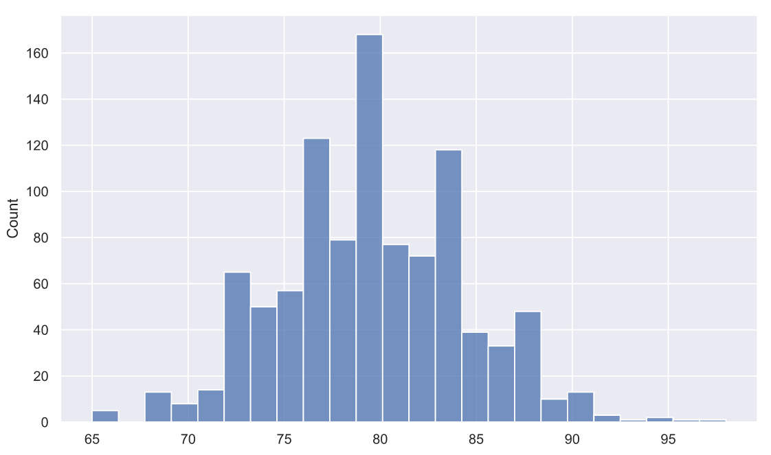
, , . 80 5 . , , , , , - .
, . , - . , - , ? - . , 10 , :
![[89, 99, 93, 84, 79, 61, 82, 81, 87, 82]](https://habrastorage.org/getpro/habr/upload_files/111/47c/b45/11147cb4509f3d49e1c731d87a8b657b.svg)
Z- :

 - ,
- , 
 ,
,  - . :
- . :
sample = np.array([89,99,93,84,79,61,82,81,87,82])
sample.mean()
83.7
Z-:
z = 10**0.5*(sample.mean()-80)/5
z
2.340085468524603
p-value:
1 - (stats.norm.cdf(z) - stats.norm.cdf(-z))
0.019279327322753836
, , : Z- 0 2 , .. 10 , , , 0.02. , 10 , ""  , , 10 "" 83.7 2%. , , , , . .
- 10 , , :
sample.std(ddof=1)
10.055954565441423
ddof std
 , ,
, ,  , . :
, . :

, ,  . -
. - 
 ,
, 
 .
. 
 ? ,
? , 
 -
-  ,
,  .
.  , - .
, - .
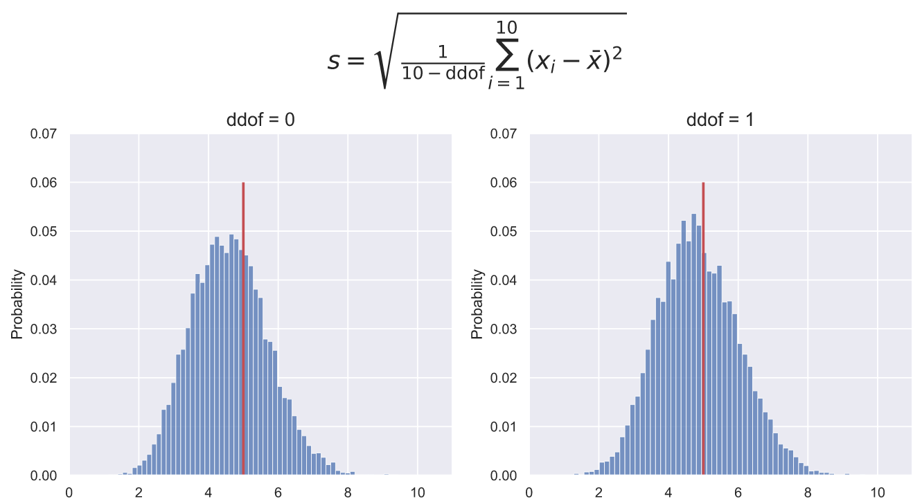
, std() NumPy ddof, 0, std() , , ddof=1. . , 10000 10  , , ddof=0 . ddof=1 , - , ddof=0:
fig, ax = plt.subplots(nrows=1, ncols=2, figsize = (12, 5))
for i in [0, 1]:
deviations = np.std(stats.norm.rvs(80, 5, (10000, 10)), axis=1, ddof=i)
sns.histplot(x=deviations ,stat='probability', ax=ax[i])
ax[i].vlines(5, 0, 0.06, color='r', lw=2)
ax[i].set_title('ddof = ' + str(i), fontsize = 15)
ax[i].set_ylim(0, 0.07)
ax[i].set_xlim(0, 11)
fig.suptitle(r'$s={\sqrt {{\frac {1}{10 - \mathrm{ddof}}}\sum _{i=1}^{10}\left(x_{i}-{\bar {x}}\right)^{2}}}$',
fontsize = 20, y=1.15);
, Z-? , - , . 5000 10 ,  :
:
deviations = np.std(stats.norm.rvs(80, 5, (5000, 10)), axis=1, ddof=1)
sns.histplot(x=deviations ,stat='probability');

, , 10- . . , , 10 2%, , ( ) 10 0. , , : 10- , .
, , , : - , - , . , ""  , Z- p-value 10- :
z = 10**0.5*(sample.mean()-80)/10
p = 1 - (stats.norm.cdf(z) - stats.norm.cdf(-z))
print(f'z = {z:.3}')
print(f'p-value = {p:.4}')
z = 1.17
p-value = 0.242
,  , , , .. ,
  , . 2%, 25%. , -
 .
.
, ? ! , : (, , - )

T-, Z- ,  ,
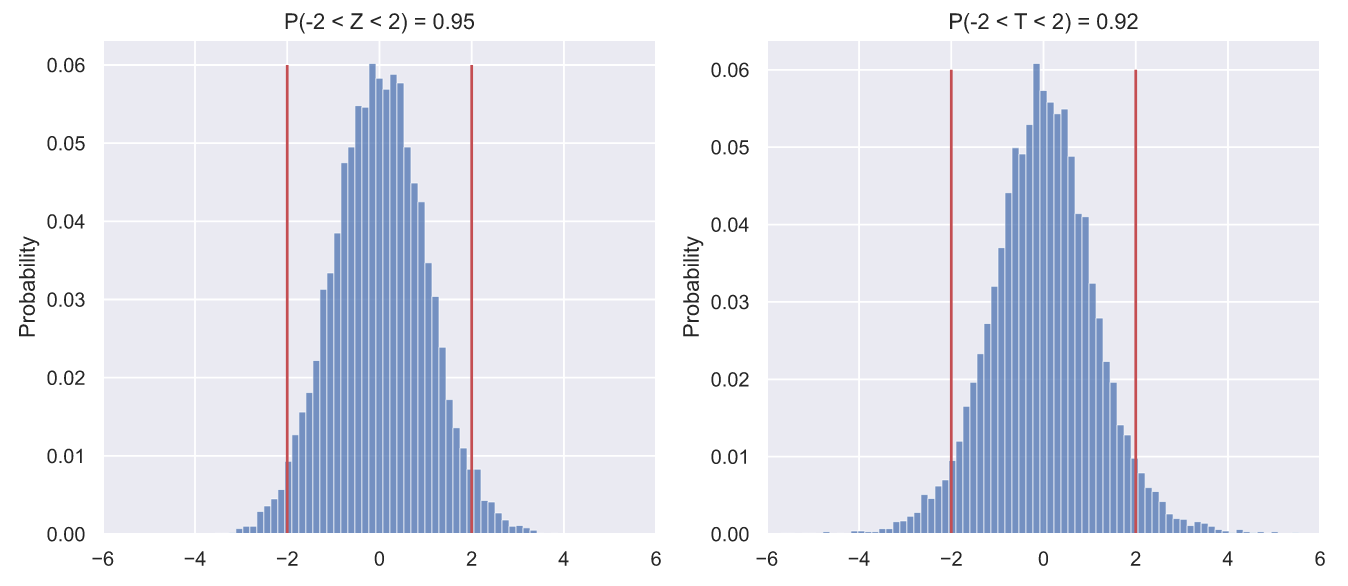
,  . 10000
  , Z- T-, :
fig, ax = plt.subplots(nrows=1, ncols=2, figsize = (12, 5))
N = 10000
samples = stats.norm.rvs(80, 5, (N, 10))
statistics = [lambda x: 10**0.5*(np.mean(x, axis=1) - 80)/5,
lambda x: 10**0.5*(np.mean(x, axis=1) - 80)/np.std(x, axis=1, ddof=1)]
title = 'ZT'
bins = np.linspace(-6, 6, 80, endpoint=True)
for i in range(2):
values = statistics[i](samples)
sns.histplot(x=values ,stat='probability', bins=bins, ax=ax[i])
p = values[(values > -2)&(values < 2)].size/N
ax[i].set_title('P(-2 < {} < 2) = {:.3}'.format(title[i], p))
ax[i].set_xlim(-6, 6)
ax[i].vlines([-2, 2], 0, 0.06, color='r');
- :
import matplotlib.animation as animation
fig, axes = plt.subplots(nrows=1, ncols=2, figsize = (18, 8))
def animate(i):
for ax in axes:
ax.clear()
N = 10000
samples = stats.norm.rvs(80, 5, (N, 10))
statistics = [lambda x: 10**0.5*(np.mean(x, axis=1) - 80)/5,
lambda x: 10**0.5*(np.mean(x, axis=1) - 80)/np.std(x, axis=1, ddof=1)]
title = 'ZT'
bins = np.linspace(-6, 6, 80, endpoint=True)
for j in range(2):
values = statistics[j](samples)
sns.histplot(x=values ,stat='probability', bins=bins, ax=axes[j])
p = values[(values > -2)&(values < 2)].size/N
axes[j].set_title(r'$P(-2\sigma < {} < 2\sigma) = {:.3}$'.format(title[j], p))
axes[j].set_xlim(-6, 6)
axes[j].set_ylim(0, 0.07)
axes[j].vlines([-2, 2], 0, 0.06, color='r')
return axes
dist_animation = animation.FuncAnimation(fig,
animate,
frames=np.arange(7),
interval = 200,
repeat = False)
dist_animation.save('statistics_dist.gif',
writer='imagemagick',
fps=1)
, , . ? -, , . , , ? , , 
![[-2 \ sigma; 2 \ sigma]](https://habrastorage.org/getpro/habr/upload_files/f0d/a1c/cfd/f0da1ccfdb352631a44937d502801011.svg) 95.5% . Z- , T- , 92-93% . , , - , :
95.5% . Z- , T- , 92-93% . , , - , :
statistics = [lambda x: 10**0.5*(np.mean(x, axis=1) - 80)/5,
lambda x: 10**0.5*(np.mean(x, axis=1) - 80)/np.std(x, axis=1, ddof=1)]
quantity = 50
N=10000
result = []
for i in range(quantity):
samples = stats.norm.rvs(80, 5, (N, 10))
Z = statistics[0](samples)
p_z = Z[(Z > -2)&((Z < 2))].size/N
T = statistics[1](samples)
p_t = T[(T > -2)&((T < 2))].size/N
result.append([p_z, p_t])
result = np.array(result)
fig, ax = plt.subplots()
line1, line2 = ax.plot(np.arange(quantity), result)
ax.legend([line1, line2],
[r'$P(-2\sigma < {} < 2\sigma)$'.format(i) for i in 'ZT'])
ax.hlines(result.mean(axis=0), 0, 50, color='0.6');
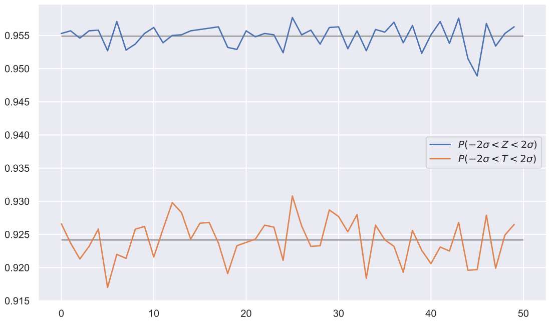
50 . , , , , . ? , ! Z- T- , . , T- ? , - . , , - , , , . , . , - , , 
 .
.
Z-,  ,
,  - . 10000
  10 , :
# ,
# svg png:
#%config InlineBackend.figure_format = 'png'
N = 10000
samples = stats.norm.rvs(80, 5, (N, 10))
means = samples.mean(axis=1)
deviations = samples.std(ddof=1, axis=1)
T = statistics[1](samples)
P = (T > -2)&((T < 2))
fig, ax = plt.subplots()
ax.scatter(means[P], deviations[P], c='b', alpha=0.7,
label=r'$\left | T \right | < 2\sigma$')
ax.scatter(means[~P], deviations[~P], c='r', alpha=0.7,
label=r'$\left | T \right | > 2\sigma$')
mean_x = np.linspace(75, 85, 300)
s = np.abs(10**0.5*(mean_x - 80)/2)
ax.plot(mean_x, s, color='k',
label=r'$\frac{\sqrt{n}(\bar{x}-\mu)}{2}$')
ax.legend(loc = 'upper right', fontsize = 15)
ax.set_title(' \n ',
fontsize=15)
ax.set_xlabel(r' ($\bar{x}$)',
fontsize=15)
ax.set_ylabel(r' ($s$)',
fontsize=15);
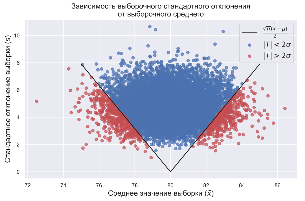
, . , , 
 , .. . , ,
  ,
, 
 . , ( ) , :

,  , .. , , ,
  ,
,  :
:

, ![[-2\sigma; 2\sigma]](https://habrastorage.org/getpro/habr/upload_files/bea/828/453/bea828453e4b32cb920e5d40a188262d.svg) , , 92,5% .
, , 92,5% .
? , . , ( ) 100- . , , ( ). 10- 82- , 2- . , , .  , , ..
  ? Z-:
? Z-:

 p-value:
z = 10**0.5*(82-80)/2
p = 1 - (stats.norm.cdf(z) - stats.norm.cdf(-z))
print(f'p-value = {p:.2}')
p-value = 0.0016
10 82- 2%.  . ,
. ,  , , , .
, , , . (  ) (
) (  ).
).
10 . 82 , , , 9- . ? :
z = 10**0.5*(82-80)/9
p = 1 - (stats.norm.cdf(z) - stats.norm.cdf(-z))
print(f'p-value = {p:.2}')
p-value = 0.48
10 

 . , , - .
, , . :
import matplotlib.animation as animation
fig, ax = plt.subplots(figsize = (15, 9))
def animate(i):
ax.clear()
N = 10000
samples = stats.norm.rvs(80, 5, (N, i))
means = samples.mean(axis=1)
deviations = samples.std(ddof=1, axis=1)
T = i**0.5*(np.mean(samples, axis=1) - 80)/np.std(samples, axis=1, ddof=1)
P = (T > -2)&((T < 2))
prob = T[P].size/N
ax.set_title(r' $s$ $\bar{x}$ $n = $' + r'${}$'.format(i),
fontsize = 20)
ax.scatter(means[P], deviations[P], c='b', alpha=0.7,
label=r'$\left | T \right | < 2\sigma$')
ax.scatter(means[~P], deviations[~P], c='r', alpha=0.7,
label=r'$\left | T \right | > 2\sigma$')
mean_x = np.linspace(75, 85, 300)
s = np.abs(i**0.5*(mean_x - 80)/2)
ax.plot(mean_x, s, color='k',
label=r'$\frac{\sqrt{n}(\bar{x}-\mu)}{2}$')
ax.legend(loc = 'upper right', fontsize = 15)
ax.set_xlim(70, 90)
ax.set_ylim(0, 10)
ax.set_xlabel(r' ($\bar{x}$)',
fontsize='20')
ax.set_ylabel(r' ($s$)',
fontsize='20')
return ax
dist_animation = animation.FuncAnimation(fig,
animate,
frames=np.arange(5, 21),
interval = 200,
repeat = False)
dist_animation.save('sigma_rel.gif',
writer='imagemagick',
fps=3)

, 


 , .
, .  Z-,
Z-,  .
.
! , ? - , , . , , 10- :
![[89,99,93,84,79,61,82,81,87,82]](https://habrastorage.org/getpro/habr/upload_files/e5d/05a/011/e5d05a011425a07da6167192fdea7c18.svg)
 ,
,  , , , , ,
  . Z-, T-, Z- ,
 . , -
. , -  ,
,  - ?
- ?  ?: ,
?: ,  ,
,  ,
, 
 ?
?
, . , - . ,  , , , 10 , 10 . ,
  . , - , .
:  ,
,  ,
, 
 . , ,
. , , 
 :
:
N = 10000
sigma = np.linspace(5, 20, 151)
prob = []
for i in sigma:
p = []
for j in range(10):
samples = stats.norm.rvs(80, i, (N, 10))
means = samples.mean(axis=1)
deviations = samples.std(ddof=1, axis=1)
p_m = means[(means >= 83) & (means <= 84)].size/N
p_d = deviations[(deviations >= 9.5) & (deviations <= 10.5)].size/N
p.append(p_m*p_d)
prob.append(sum(p)/len(p))
prob = np.array(prob)
fig, ax = plt.subplots()
ax.plot(sigma, prob)
ax.set_xlabel(r' ($\sigma$)',
fontsize=20)
ax.set_ylabel('',
fontsize=20);
,  . , ,
. , ,  ,
,  . - , , , , . .
T-?
, - - . 1% , - . , , . , - -. ?
- ! , - , "" t-. , , , . , , 1943 , 50% . , - .
, "" . , ( !) , "" , :

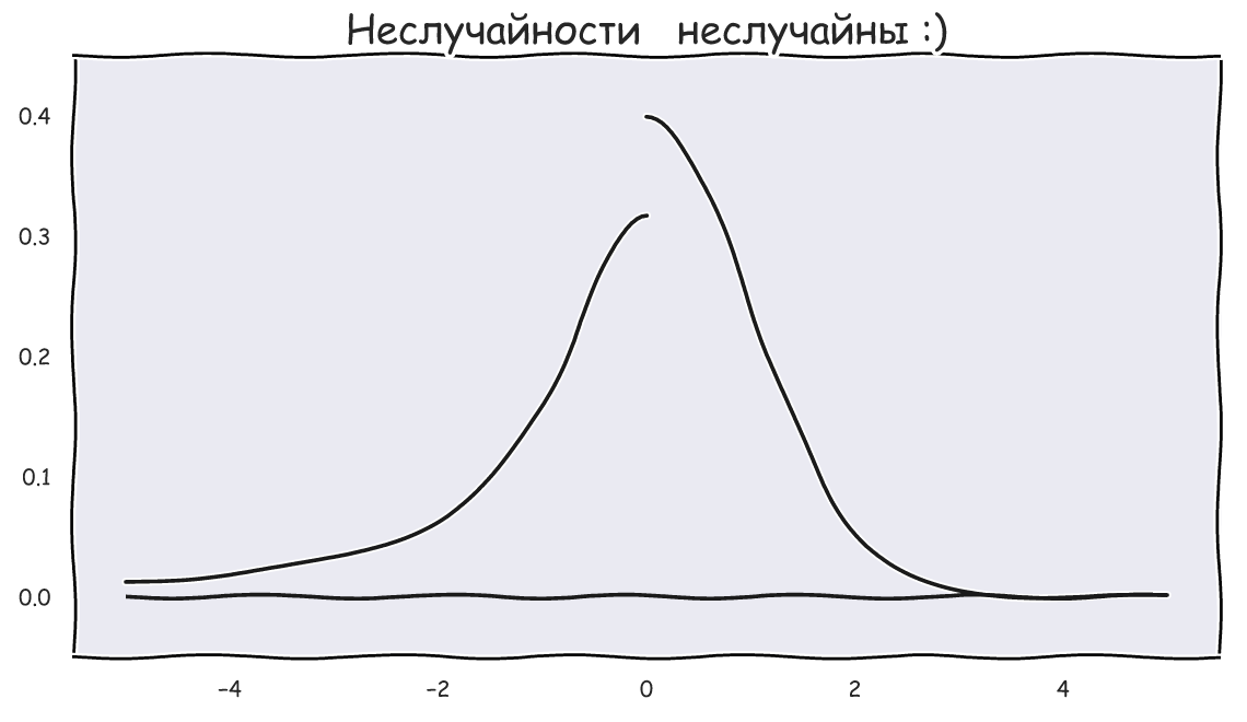
t-, . , , "", , , , , - . " ", "t-" , .
:

" " .  , ..
, ..  ,
,  , .. , . - , :

, :
import matplotlib.animation as animation
fig, ax = plt.subplots(figsize = (15, 9))
def animate(i):
ax.clear()
N = 15000
x = np.linspace(-5, 5, 100)
ax.plot(x, stats.norm.pdf(x, 0, 1), color='r')
samples = stats.norm.rvs(0, 1, (N, i))
t = samples[:, 0]/np.sqrt(np.mean(samples[:, 1:]**2, axis=1))
t = t[(t>-5)&(t<5)]
sns.histplot(x=t, bins=np.linspace(-5, 5, 100), stat='density', ax=ax)
ax.set_title(r' $t(n)$ n = ' + str(i), fontsize = 20)
ax.set_xlim(-5, 5)
ax.set_ylim(0, 0.5)
return ax
dist_animation = animation.FuncAnimation(fig,
animate,
frames=np.arange(2, 21),
interval = 200,
repeat = False)
dist_animation.save('t_rel_of_df.gif',
writer='imagemagick',
fps=3)
,  , , ,
, , ,  . , , :

SciPy:
import matplotlib.animation as animation
fig, ax = plt.subplots(figsize = (15, 9))
def animate(i):
ax.clear()
N = 15000
x = np.linspace(-5, 5, 100)
ax.plot(x, stats.norm.pdf(x, 0, 1), color='r')
ax.plot(x, stats.t.pdf(x, df=i))
ax.set_title(r' $t(n)$ n = ' + str(i), fontsize = 20)
ax.set_xlim(-5, 5)
ax.set_ylim(0, 0.45)
return ax
dist_animation = animation.FuncAnimation(fig,
animate,
frames=np.arange(2, 21),
interval = 200,
repeat = False)
dist_animation.save('t_pdf_rel_of_df.gif',
writer='imagemagick',
fps=3)

,  ( df ) . - , ,
  , .
, .
t-
t- SciPy :
sample = np.array([89,99,93,84,79,61,82,81,87,82])
stats.ttest_1samp(sample, 80)
Ttest_1sampResult(statistic=1.163532240174695, pvalue=0.2745321678073461)
:
T = 9**0.5*(sample.mean() -80)/sample.std()
T
1.163532240174695
,  ,
,  ,
,  . , 1 , , , . :
T = 10**0.5*(sample.mean() -80)/sample.std(ddof=1)
T
1.1635322401746953
, t- , p-value? , - , p-value Z-, t-:
t = stats.t(df=9)
fig, ax = plt.subplots()
x = np.linspace(t.ppf(0.001), t.ppf(0.999), 300)
ax.plot(x, t.pdf(x))
ax.hlines(0, x.min(), x.max(), lw=1, color='k')
ax.vlines([-T, T], 0, 0.4, color='g', lw=2)
x_le_T, x_ge_T = x[x<-T], x[x>T]
ax.fill_between(x_le_T, t.pdf(x_le_T), np.zeros(len(x_le_T)), alpha=0.3, color='b')
ax.fill_between(x_ge_T, t.pdf(x_ge_T), np.zeros(len(x_ge_T)), alpha=0.3, color='b')
p = 1 - (t.cdf(T) - t.cdf(-T))
ax.set_title(r'$P(\left | T \right | \geqslant {:.3}) = {:.3}$'.format(T, p));

, p-value 27%, .. , - ,  , p-value , 5 . , , - ,
  , 0.95:

SciPy, interval loc () scale () :
sample_loc = sample.mean()
sample_scale = sample.std(ddof=1)/10**0.5
ci = stats.t.interval(0.95, df=9, loc=sample_loc, scale=sample_scale)
ci
(76.50640345566619, 90.89359654433382)
,  , ,
, , 
![[76,5; 90,9]](https://habrastorage.org/getpro/habr/upload_files/271/4c8/21d/2714c821d6a7a520116d1a2df7c3059c.svg) . , ,
. , ,  , .
, .
, , , ( ). , , t- , t- , t- .
Por supuesto, me gustaría insertar algún gif al final, pero quiero terminar con la frase de Herbert Spencer: " El mayor objetivo de la educación no es el conocimiento, sino la acción ", ¡así que lanza tus anacondas y actúa! Esto es especialmente cierto para las personas autodidactas como yo.
¡Presiono F5 y espero sus comentarios!