La traducción se preparó como parte del curso " Machine Learning. Basic ".
Invitamos a todos los participantes al intensivo en línea abierto "Ciencia de datos: es más fácil de lo que parece" . Hablemos de la historia y los hitos en el desarrollo de la IA, descubrirás qué tareas resuelve DS y qué hace ML. Y ya en la primera lección, podrás enseñarle a la computadora a determinar qué se muestra en la imagen. Es decir, intentará entrenar su primer modelo de aprendizaje automático para resolver un problema de clasificación de imágenes. Créame, ¡es más fácil de lo que parece!
¿No está seguro de qué herramienta de visualización utilizar? En este artículo, detallaremos los pros y los contras de cada biblioteca.
Python, :
Matplotlib
Seaborn
Plotly
Bokeh
Altair
Folium
DataFrame? . . , .
, , :
, ?
, Matplotlib, , ( , ).
, Altair, Bokeh Plotly, , , .
? , Matplotlib, , , API. , Altair, , .
, , , , ?
, Github :
I Scraped more than 1k Top Machine Learning Github Profiles and this is what I Found
Datapane, Python API Python-. Datapane.
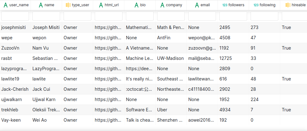
csv , Datapane Blob.
import datapane as dp
dp.Blob.get(name='github_data', owner='khuyentran1401').download_df()
Datapane, Blob. .
Matplotlib
Matplotlib, , Python . , data science, Matplotlib.
.
, 100 , Matplotlib :
import matplotlib.pyplot as plt
top_followers = new_profile.sort_values(by='followers', axis=0, ascending=False)[:100]
fig = plt.figure()
plt.bar(top_followers.user_name,
top_followers.followers)
- :
fig = plt.figure()
plt.text(0.6, 0.7, "learning", size=40, rotation=20.,
ha="center", va="center",
bbox=dict(boxstyle="round",
ec=(1., 0.5, 0.5),
fc=(1., 0.8, 0.8),
)
)
plt.text(0.55, 0.6, "machine", size=40, rotation=-25.,
ha="right", va="top",
bbox=dict(boxstyle="square",
ec=(1., 0.5, 0.5),
fc=(1., 0.8, 0.8),
)
)
plt.show()
Matplotlib , , .
, , , X Y, , Matplotlib .
correlation = new_profile.corr()
fig, ax = plt.subplots()
im = plt.imshow(correlation)
ax.set_xticklabels(correlation.columns)
ax.set_yticklabels(correlation.columns)
plt.setp(ax.get_xticklabels(), rotation=45, ha="right",
rotation_mode="anchor")
: Matplotlib , , .
Seaborn
Seaborn - Python , Matplotlib. , .
. , seaborn , matplotlib, .
, , .
correlation = new_profile.corr()
sns.heatmap(correlation, annot=True)
x y!
2.
seaborn , , , . ., , , . , , Matplotlib.
sns.set(style="darkgrid")
titanic = sns.load_dataset("titanic")
ax = sns.countplot(x="class", data=titanic)
Seaborn , matplotlib.
: Seaborn — Matplotlib . , , Matplotlib, seaborn (, , , . .), .
Plotly
Python Plotly . , Matplotlib seaborn, , , , . .
R
R Python, Plotly Python!
- Plotly Express, Python.
import plotly.express as px
fig = px.scatter(new_profile[:100],
x='followers',
y='total_stars',
color='forks',
size='contribution')
fig.show()
2.
Plotly . , .
, matplotlib? , Plotly
import plotly.express as px
top_followers = new_profile.sort_values(by='followers', axis=0, ascending=False)[:100]
fig = px.bar(top_followers,
x='user_name',
y='followers',
)
fig.show()
, , , . , .
3.
Plotly .
import plotly.express as px
import datapane as dp
location_df = dp.Blob.get(name='location_df', owner='khuyentran1401').download_df()
m = px.scatter_geo(location_df, lat='latitude', lon='longitude',
color='total_stars', size='forks',
hover_data=['user_name','followers'],
title='Locations of Top Users')
m.show()
, , . , - .
: Plotly .
Altair
Altair - Python , vega-lite, , .
1.
, , . , . , , , .
, . , , count() y_axis
import seaborn as sns
import altair as alt
titanic = sns.load_dataset("titanic")
alt.Chart(titanic).mark_bar().encode(
alt.X('class'),
y='count()'
)
2.
Altair .
, , , Plotly, Altair , .
hireable = alt.Chart(titanic).mark_bar().encode(
x='sex:N',
y='mean_age:Q'
).transform_aggregate(
mean_age='mean(age)',
groupby=['sex'])
hireable
, transform_aggregate()
(mean(age)
) (groupby=['sex']
) mean_age
). Y .
, - ( ), :N
, mean_age
- ( , ), :Q
.
3.
Altair , , .
, , . - :
brush = alt.selection(type='interval')
points = alt.Chart(titanic).mark_point().encode(
x='age:Q',
y='fare:Q',
color=alt.condition(brush, 'class:N', alt.value('lightgray'))
).add_selection(
brush
)
bars = alt.Chart(titanic).mark_bar().encode(
y='class:N',
color='class:N',
x = 'count(class):Q'
).transform_filter(
brush
)
points & bars
, , . , , , , - Python!
, , , , , , seaborn Plotly. Altair 5000 .
: Altair . Altair , 5000 , Plotly Seaborn.
Bokeh
Bokeh - , .
Matplotlib
, Bokeh, , Matplotlib.
Matplotlib , . Bokeh , ; , , Matplotlib, .
, Matplotlib,
import matplotlib.pyplot as plt
fig, ax = plt.subplots()
x = [1, 2, 3, 4, 5]
y = [2, 5, 8, 2, 7]
for x,y in zip(x,y):
ax.add_patch(plt.Circle((x, y), 0.5, edgecolor = "#f03b20",facecolor='#9ebcda', alpha=0.8))
#Use adjustable='box-forced' to make the plot area square-shaped as well.
ax.set_aspect('equal', adjustable='datalim')
ax.set_xbound(3, 4)
ax.plot() #Causes an autoscale update.
plt.show()
, Bokeh, :
from bokeh.io import output_file, show
from bokeh.models import Circle
from bokeh.plotting import figure
reset_output()
output_notebook()
plot = figure(plot_width=400, plot_height=400, tools="tap", title="Select a circle")
renderer = plot.circle([1, 2, 3, 4, 5], [2, 5, 8, 2, 7], size=50)
selected_circle = Circle(fill_alpha=1, fill_color="firebrick", line_color=None)
nonselected_circle = Circle(fill_alpha=0.2, fill_color="blue", line_color="firebrick")
renderer.selection_glyph = selected_circle
renderer.nonselection_glyph = nonselected_circle
show(plot)
2.
Bokeh . , , .
, 3 ,
from bokeh.layouts import gridplot, row
from bokeh.models import ColumnDataSource
reset_output()
output_notebook()
source = ColumnDataSource(new_profile)
TOOLS = "box_select,lasso_select,help"
TOOLTIPS = [('user', '@user_name'),
('followers', '@followers'),
('following', '@following'),
('forks', '@forks'),
('contribution', '@contribution')]
s1 = figure(tooltips=TOOLTIPS, plot_width=300, plot_height=300, title=None, tools=TOOLS)
s1.circle(x='followers', y='following', source=source)
s2 = figure(tooltips=TOOLTIPS, plot_width=300, plot_height=300, title=None, tools=TOOLS)
s2.circle(x='followers', y='forks', source=source)
s3 = figure(tooltips=TOOLTIPS, plot_width=300, plot_height=300, title=None, tools=TOOLS)
s3.circle(x='followers', y='contribution', source=source)
p = gridplot([[s1,s2,s3]])
show(p)
Bokeh - , , , Matplotlib, , Seaborn, Altair Plotly.
, , , , .
, :
from bokeh.transform import factor_cmap
from bokeh.palettes import Spectral6
p = figure(x_range=list(titanic_groupby['class']))
p.vbar(x='class', top='survived', source = titanic_groupby,
fill_color=factor_cmap('class', palette=Spectral6, factors=list(titanic_groupby['class'])
))
show(p)
, , :
from bokeh.transform import factor_cmap
from bokeh.palettes import Spectral6
p = figure(x_range=list(titanic_groupby['class']))
p.vbar(x='class', top='survived', width=0.9, source = titanic_groupby,
fill_color=factor_cmap('class', palette=Spectral6, factors=list(titanic_groupby['class'])
))
show(p)
, , Bokeh
: Bokeh - , , , . , , , .
Folium
Folium . OpenStreetMap
, Mapbox Stamen
, Plotly, Altair Bokeh , Folium , - Google Map,
, Github Plotly? Folium:
import folium
# Load data
location_df = dp.Blob.get(name='location_df', owner='khuyentran1401').download_df()
# Save latitudes, longitudes, and locations' names in a list
lats = location_df['latitude']
lons = location_df['longitude']
names = location_df['location']
# Create a map with an initial location
m = folium.Map(location=[lats[0], lons[0]])
for lat, lon, name in zip(lats, lons, names):
# Create marker with other locations
folium.Marker(location=[lat, lon],
popup= name,
icon=folium.Icon(color='green')
).add_to(m)
m
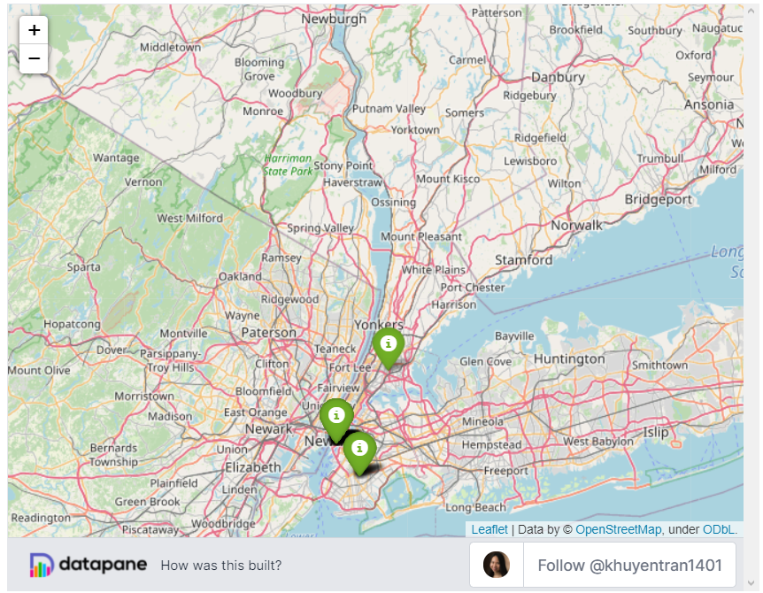
2.
, Folium , :
# Code to generate map here
#....
# Enable adding more locations in the map
m = m.add_child(folium.ClickForMarker(popup='Potential Location'))
, , , .
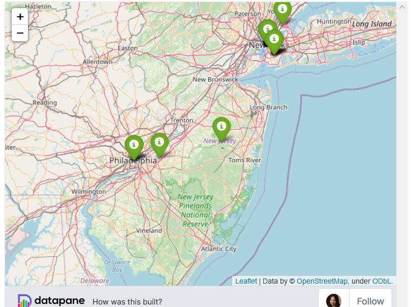
3.
Folium , , Altair. , Github , , Github ? Folium :
from folium.plugins import HeatMap
m = folium.Map(location=[lats[0], lons[0]])
HeatMap(data=location_df[['latitude', 'longitude', 'total_stars']]).add_to(m)
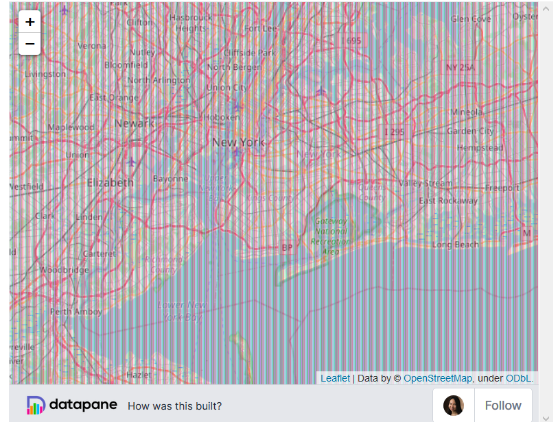
, .
: Folium . Google Map.
! . , . .
, , , . , , , !
data science . LinkedIn Twitter.