Las fechas y los horarios no son objetos fáciles:
- los meses contienen un número diferente de días;
- los años son bisiestos y no;
- hay diferentes zonas horarias;
- las horas, los minutos y los días utilizan diferentes sistemas numéricos;
- y muchos otros matices.
El siguiente es un resumen de algunos puntos que rara vez se destacan en la documentación, así como trucos que le permiten escribir código rápido y controlado.
Un resumen muy breve para lectores de teléfonos inteligentes: en grandes cantidades de datos, usamos solo una POSIXct
fracción de segundo. Será bueno, por supuesto, rápido.
Es una continuación de una serie de publicaciones anteriores .
Estándares para especificar fechas y horas
ISO 8601 Elementos de datos y formatos de intercambio - Intercambio de información - La representación de fechas y horas es un estándar internacional que cubre el intercambio de datos relacionados con la fecha y la hora.
Métodos básicos de R para trabajar con el tiempo
fecha
Sys.Date()
print("-----")
x <- as.Date("2019-01-29") # UTC
print(x)
tz(x)
str(x)
dput(x)
print("-----")
dput(as.Date("1970-01-01")) # ! origin
## [1] "2021-04-29" ## [1] "-----" ## [1] "2019-01-29" ## [1] "UTC" ## Date[1:1], format: "2019-01-29" ## structure(17925, class = "Date") ## [1] "-----" ## structure(0, class = "Date")
El formato de fecha no estándar durante la inicialización debe especificarse especialmente
as.Date("04/20/2011", format = "%m/%d/%Y")
## [1] "2011-04-20"
Hora
Hay dos tipos básicos de tiempo usados en R: POSIXct
y POSIXlt
.
Las vistas externas POSIXct
y se POSIXlt
ven similares. ¿Y los internos?
z <- Sys.time()
glue(" ",
"POSIXct - {z}",
"POSIXlt - {as.POSIXlt(z)}", "---", .sep = "\n")
glue(" ",
"POSIXct - {capture.output(dput(z))}",
"POSIXlt - {paste0(capture.output(dput(as.POSIXlt(z))), collapse = '')}",
"---", .sep = "\n")
# /
glue(": {year(z)} \n: {minute(z)}\n: {second(z)}\n---")
## ## POSIXct - 2021-04-29 15:18:04 ## POSIXlt - 2021-04-29 15:18:04 ## --- ## ## POSIXct - structure(1619698684.50764, class = c("POSIXct", "POSIXt")) ## POSIXlt - structure(list(sec = 4.50764489173889, min = 18L, hour = 15L, mday = 29L, mon = 3L, year = 121L, wday = 4L, yday = 118L, isdst = 0L, zone = "MSK", gmtoff = 10800L), class = c("POSIXlt", "POSIXt"), tzone = c("", "MSK", "MSD")) ## --- ## : 2021 ## : 18 ## : 4 ## ---
Inmediatamente concluimos que para un trabajo serio con datos (más de 10 líneas con el tiempo), lo POSIXlt
olvidamos como un mal sueño. Es una estructura compleja con una sobrecarga loca.
POSIXct
unixtimestamp, () ( 0 01.01.1970). .
— online unixtimestamp:
- Epoch Unix Time Stamp Converter
- Epoch & Unix Timestamp Conversion Tools
- currentDate / Time in Millisecondsmillis
z <- 1548802400
as.POSIXct(z, origin = "1970-01-01") # local
as.POSIXct(z, origin = "1970-01-01", tz = "UTC") # in UTC
## [1] "2019-01-30 01:53:20 MSK" ## [1] "2019-01-29 22:53:20 UTC"
. . :
- ISO, (ISO 8601-2019);
- - ;
- .
POSIXct
, - . :
x <- ymd_hms("2014-09-24 15:23:10")
x
x + 0.5
x + 0.5 + 0.6
options(digits.secs=5)
x + 0.45756
options(digits.secs=0)
x
## [1] "2014-09-24 15:23:10 UTC" ## [1] "2014-09-24 15:23:10 UTC" ## [1] "2014-09-24 15:23:11 UTC" ## [1] "2014-09-24 15:23:10.45756 UTC" ## [1] "2014-09-24 15:23:10 UTC"
, .
options(digits.secs=5)
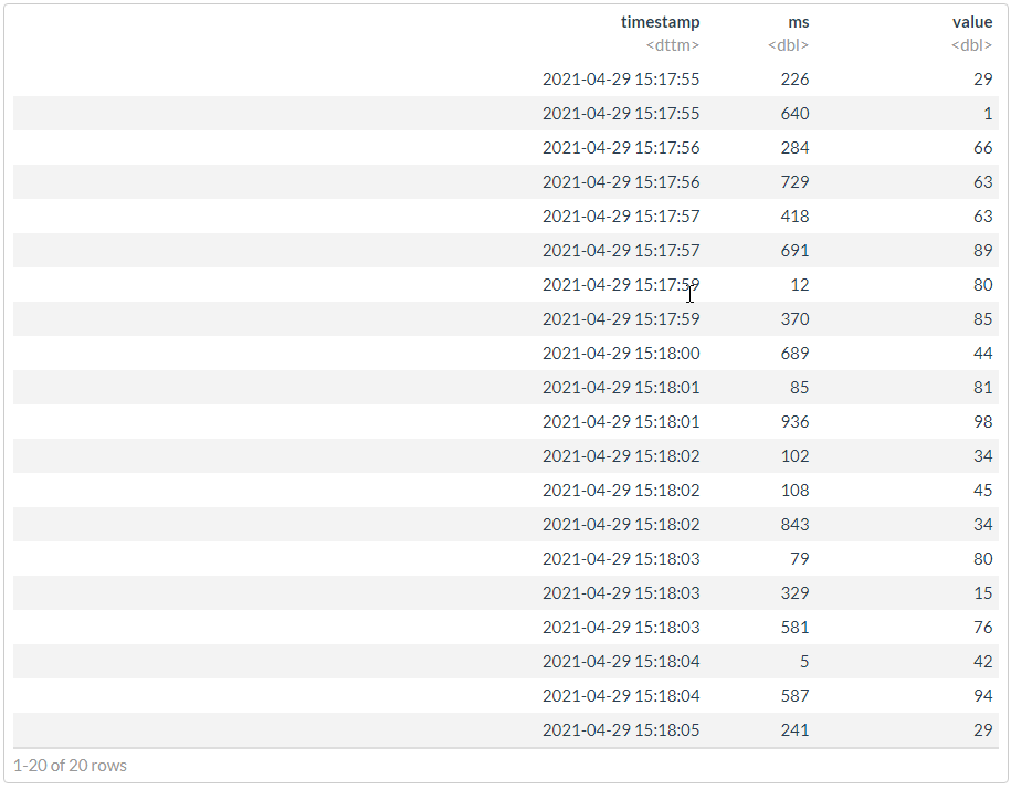
# generate data
df <- data.frame(
timestamp = as_datetime(
round(runif(20, min = now() - seconds(10), max = now()), 0),
tz ="Europe/Moscow")) %>%
mutate(ms = round(runif(n(), 0, 999), 0)) %>%
mutate(value = round(runif(n(), 0, 100), 0))
dput(df)
# " "
df %>%
arrange(timestamp, ms)
options(digits.secs=0)
## structure(list(timestamp = structure(c(1619698677, 1619698680, ## 1619698676, 1619698682, 1619698675, 1619698682, 1619698679, 1619698679, ## 1619698684, 1619698683, 1619698684, 1619698677, 1619698682, 1619698683, ## 1619698675, 1619698676, 1619698685, 1619698681, 1619698683, 1619698681 ## ), class = c("POSIXct", "POSIXt"), tzone = "Europe/Moscow"), ## ms = c(418, 689, 729, 108, 226, 843, 12, 370, 5, 581, 587, ## 691, 102, 79, 640, 284, 241, 85, 329, 936), value = c(63, ## 44, 63, 45, 29, 34, 80, 85, 42, 76, 94, 89, 34, 80, 1, 66, ## 29, 81, 15, 98)), class = "data.frame", row.names = c(NA, ## -20L))
# ""
# [magrittr aliases](https://magrittr.tidyverse.org/reference/aliases.html)
df2 <- df %>%
mutate(timestamp = timestamp + ms/1000) %>%
# mutate_at("timestamp", ~`+`(. + ms/1000)) %>%
select(-ms) %>%
df2 %>% arrange(timestamp)

#
dt <- as.data.table(df2)
bench::mark(
naive = dplyr::arrange(df, timestamp, ms),
smart = dplyr::arrange(df2, timestamp),
dt = dt[order(timestamp)],
check = FALSE,
relative = TRUE,
min_iterations = 1000
)
## # A tibble: 3 x 6 ## expression min median `itr/sec` mem_alloc `gc/sec` ## <bch:expr> <dbl> <dbl> <dbl> <dbl> <dbl> ## 1 naive 11.9 11.8 1 1.06 1 ## 2 smart 11.1 11.0 1.06 1 1.06 ## 3 dt 1 1 11.6 494. 1.22
.
data <- c("05102019210003657", "05102019210003757", "05102019210003857")
dmy_hms(stri_c(stri_sub(data, to = 14L), ".", stri_sub(data, from = 15L)), tz = "Europe/Moscow")
#
data2 <- data %>%
sample(10^6, replace = TRUE)
bench::mark(
stri_sub = stri_c(stri_sub(data2, to = 14L), ".", stri_sub(data2, from = 15L)),
stri_replace = stri_replace_first_regex(data2, pattern = "(^.{14})(.*)", replacement = "$1.$2"),
re2_replace = re2_replace(data2, pattern = "(^.{14})(.*)", replacement = "\\1.\\2", parallel = TRUE)
)
## [1] "2019-10-05 21:00:03 MSK" "2019-10-05 21:00:03 MSK" ## [3] "2019-10-05 21:00:03 MSK" ## # A tibble: 3 x 6 ## expression min median `itr/sec` mem_alloc `gc/sec` ## <bch:expr> <bch:tm> <bch:tm> <dbl> <bch:byt> <dbl> ## 1 stri_sub 214ms 222ms 4.10 22.89MB 5.47 ## 2 stri_replace 653ms 653ms 1.53 7.63MB 0 ## 3 re2_replace 409ms 413ms 2.42 15.29MB 1.21
lubridate
x <- ymd(20101215)
print(x)
class(x)
## [1] "2010-12-15" ## [1] "Date"
lubridate
ymd(20101215) == mdy("12/15/10")
## [1] TRUE
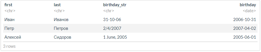
df <- tibble(first = c("", "", ""),
last = c("", "", ""),
birthday_str = c("31-10-06", "2/4/2007", "1 June, 2005")) %>%
mutate(birthday = dmy(birthday_str))
df
, ?
# lubridate
options(lubridate.verbose = TRUE)
# : ..
df <- tibble(time_str = c("08.05.19 12:04:56", "09.05.19 12:05", "12.05.19 23"))
lubridate::dmy_hms(df$time_str, tz = "Europe/Moscow")
print("---------------------")
lubridate::dmy(df$time_str, tz = "Europe/Moscow")
## [1] "2019-05-08 12:04:56 MSK" NA ## [3] NA ## [1] "---------------------" ## [1] NA NA NA
# lubridate
options(lubridate.verbose = TRUE)
lubridate::dmy_hms(df$time_str, truncated = 3, tz = "Europe/Moscow")
## [1] "2019-05-08 12:04:56 MSK" "2019-05-09 12:05:00 MSK" ## [3] "2019-05-12 23:00:00 MSK"
# lubridate
options(lubridate.verbose = TRUE)
# : ..
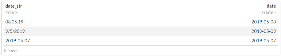
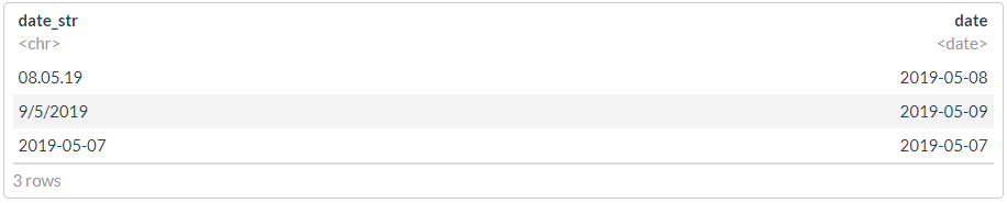
df <- tibble(date_str = c("08.05.19", "9/5/2019", "2019-05-07"))
#
glimpse(dmy(df$date_str))
print("---------------------")
#
glimpse(ymd(df$date_str))
print("---------------------")
## Date[1:3], format: "2019-05-08" "2019-05-09" NA ## [1] "---------------------" ## Date[1:3], format: "2008-05-19" NA "2019-05-07" ## [1] "---------------------"
? , , , - .
df %>% mutate(date = dplyr::coalesce(dmy(date_str), ymd(date_str)))
df1 <- df
df1$date <- dmy(df1$date_str)
idx <- is.na(df1$date)
print("---------------------")
idx
df1$date[idx] <- ymd(df1$date_str[idx])
print("---------------------")
df1
## [1] "---------------------" ## [1] FALSE FALSE TRUE ## [1] "---------------------"
"" :
POSIXct
options(lubridate.verbose = FALSE)
date1 <- ymd_hms("2011-09-23-03-45-23")
date2 <- ymd_hms("2011-10-03-21-02-19")
# ?
as.numeric(date2) - as.numeric(date1) # ,
(date2 - date1) %>% dput()
difftime(date2, date1)
difftime(date2, date1, unit="mins")
difftime(date2, date1, unit="secs")
## [1] 926216 ## structure(10.7200925925926, class = "difftime", units = "days") ## Time difference of 10.72009 days ## Time difference of 15436.93 mins ## Time difference of 926216 secs
date1 <- ymd_hms("2019-01-30 00:00:00")
date1
date1 - days(1)
date1 + days(1)
date1 + days(2)
## [1] "2019-01-30 UTC" ## [1] "2019-01-29 UTC" ## [1] "2019-01-31 UTC" ## [1] "2019-02-01 UTC"
—
date1 - months(1)
date1 + months(1) # !!!
## [1] "2018-12-30 UTC" ## [1] NA
. , .
date1 %m-% months(1)
date1 %m+% months(1)
date1 %m+% months(1) %m-% months(1)
## [1] "2018-12-30 UTC" ## [1] "2019-02-28 UTC" ## [1] "2019-01-28 UTC"
date1 <- ymd_hms("2019-01-30 01:00:00")
date1 %T>% print() %>% dput()
with_tz(date1, tzone = "Europe/Moscow") %T>% print() %>% dput()
force_tz(date1, tzone = "Europe/Moscow") %T>% print() %>% dput()
## [1] "2019-01-30 01:00:00 UTC" ## structure(1548810000, class = c("POSIXct", "POSIXt"), tzone = "UTC") ## [1] "2019-01-30 04:00:00 MSK" ## structure(1548810000, class = c("POSIXct", "POSIXt"), tzone = "Europe/Moscow") ## [1] "2019-01-30 01:00:00 MSK" ## structure(1548799200, class = c("POSIXct", "POSIXt"), tzone = "Europe/Moscow")
, , ? , hms
. .
hms_str <- "03:22:14"
as_hms(hms_str)
dput(as_hms(hms_str))
print("-------")
x <- as_hms(hms_str) * 15
x
str(x)
# seconds_to_period(period_to_seconds(x))
seconds_to_period(x) %T>% dput() %>% print()
## 03:22:14 ## structure(12134, units = "secs", class = c("hms", "difftime")) ## [1] "-------" ## Time difference of 182010 secs ## 'difftime' num 182010 ## - attr(*, "units")= chr "secs" ## new("Period", .Data = 30, year = 0, month = 0, day = 2, hour = 2, ## minute = 33) ## [1] "2d 2H 33M 30S"
— . .
( Clickhouse) , , unixtimestamp UTC. , .
:
- . timestamp, , , , , .
- ( ). , , , .
- unixtimestamp UTC , . (!).
- , timestamp. ,
X-1
X+1
, .
, 0.
.
(, ) . , :
- , ;
- ;
- ;
- ( );
- ;
-
double
; - ;
- .
-- ClickHouse
SELECT DISTINCT
store, pos,
timestamp, ms,
concat(toString(store), '-', toString(pos)) AS pos_uid,
toFloat64(timestamp) + (ms / 1000) AS timestamp
flog.info(paste("SQL query:", sql_req))
tic(" CH")
raw_df <- dbGetQuery(conn, stri_encode(sql_req, to = "UTF-8")) %>%
mutate_if(is.character, `Encoding<-`, "UTF-8") %>%
as_tibble() %>%
mutate_at(vars(timestamp), anytime::anytime, tz = "Europe/Moscow") %>%
mutate_at("event", as.factor)
flog.info(capture.output(toc()))
DBI::dbDisconnect(conn)
data.frame
#
df -> as_tibble(_df) %>%
map(pryr::object_size) %>%
unlist() %>%
enframe() %>%
arrange(desc(value)) %>%
mutate_at("value", fs::as_fs_bytes) %>%
mutate(ratio = formattable::percent(value / sum(value), 2)) %>%
add_row(name = "TOTAL", value = sum(.$value))
,
- Epoch & Unix Timestamp Conversion Tools
- currentdate/time in millisecondsmillis
- Functions for working with dates and times
, , , . .
df <- seq.Date(from = as.Date("2021-01-01"),
to = as.Date("2021-05-31"),
by = "2 days") %>%
# sample(20, replace = FALSE) %>%
tibble(date = .)
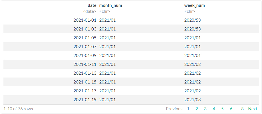
# //
# 1
df %>%
mutate(month_num = stri_c(lubridate::year(date),
sprintf("%02d", lubridate::month(date)),
sep = "/"),
week_num = stri_c(lubridate::isoyear(date),
sprintf("%02d", lubridate::isoweek(date)),
sep = "/")
)
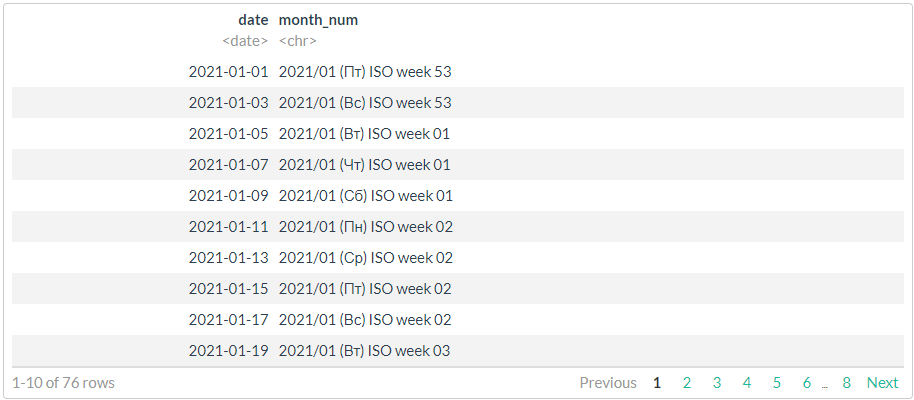
# //
# 2,
# , !!!
df %>%
mutate(month_num = format(date, "%Y/%m (%a) ISO week %V"))
# //
# 3,
# strptime (ISO 8601) ICU
# https://man7.org/linux/man-pages/man3/strptime.3.html
stri_datetime_fstr("%Y/%m (%a) week %V")
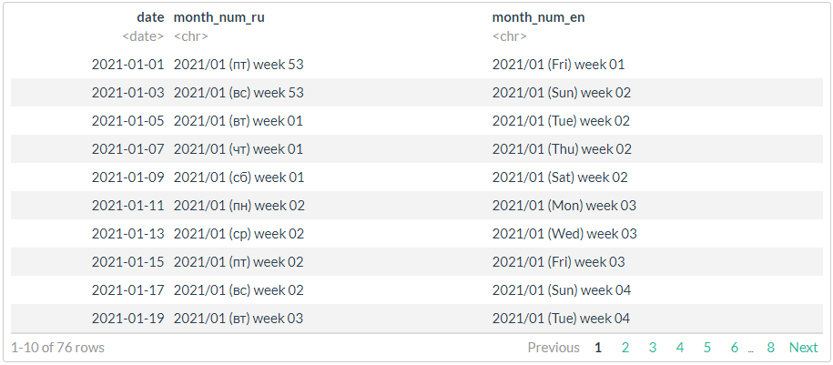
# ggthemes::tableau_color_pal("Tableau 20")(20) %>% scales::show_col()
# , !!!
df %>%
mutate(
month_num_ru = stri_datetime_format(
date, "yyyy'/'MM' ('ccc') week 'ww", locale = "ru", tz = "UTC"),
month_num_en = stri_datetime_format(
date, "yyyy'/'MM' ('ccc') week 'ww", locale = "en", tz = "UTC"))
. .
stri_datetime_format(today(), "LLLL", locale="ru@calendar=Persian")
stri_datetime_format(today(), "LLLL", locale="ru@calendar=Indian")
stri_datetime_format(today(), "LLLL", locale="ru@calendar=Hebrew")
stri_datetime_format(today(), "LLLL", locale="ru@calendar=Islamic")
stri_datetime_format(today(), "LLLL", locale="ru@calendar=Coptic")
stri_datetime_format(today(), "LLLL", locale="ru@calendar=Ethiopic")
stri_datetime_format(today(), "dd MMMM yyyy", locale="ru")
stri_datetime_format(today(), "LLLL d, yyyy", locale="ru")
## [1] "" ## [1] "" ## [1] "" ## [1] "" ## [1] "" ## [1] "" ## [1] "29 2021" ## [1] " 29, 2021"
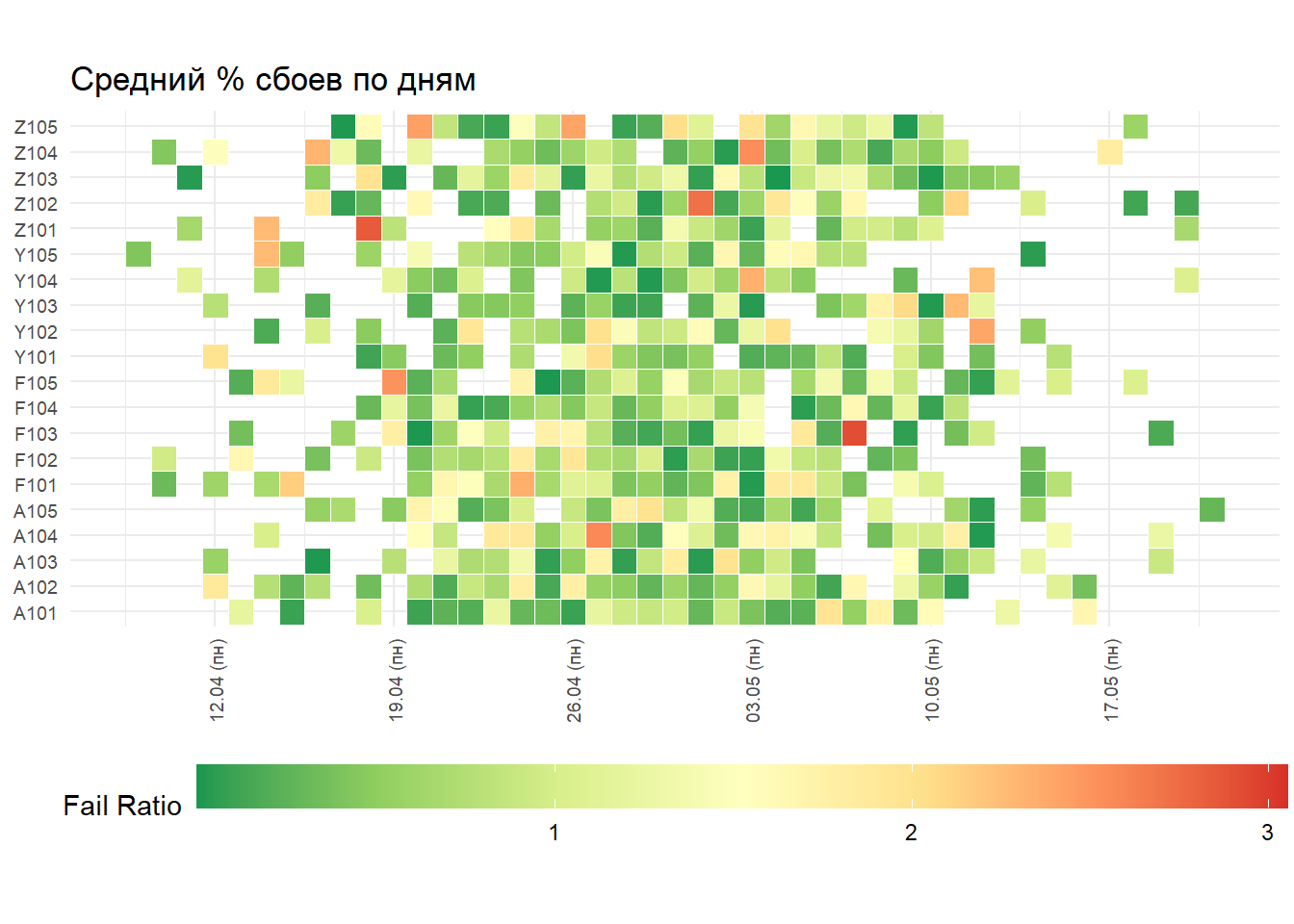
.
#
map_tbl <- tibble(
date = as_date(Sys.time() + rnorm(10^3, mean = 0, sd = 60 * 60 * 24 * 7))) %>%
mutate(store = stri_c(sample(c("A", "F", "Y", "Z"), n(), replace = TRUE),
sample(101:105, n(), replace = TRUE))) %>%
mutate(store_fct = as.factor(store)) %>%
mutate(fail_ratio = abs(rnorm(n(), mean = 0.3, sd = 1)))
my_date_format <- function (format = "dd MMMM yyyy", tz = "Europe/Moscow")
{
scales:::force_all(format, tz)
# stri_datetime_fstr("%d.%m%n%A")
# stri_datetime_fstr("%d.%m (%a)")
function(x) stri_datetime_format(x, format, locale = "ru", tz = tz)
}
# ,
gp <- map_tbl %>%
ggplot(aes(x = date, y = store_fct, fill = fail_ratio)) +
geom_tile(color = "white", size = 0.1) +
# scale_fill_distiller(palette = "RdYlGn", name = "Fail Ratio", label = comma) +
# scale_fill_distiller(palette = "RdYlGn", name = "Fail Ratio", guide = guide_legend(keywidth = unit(4, "cm"))) +
scale_fill_distiller(palette = "RdYlGn", name = "Fail Ratio") +
scale_x_date(breaks = scales::date_breaks("1 week"), labels = my_date_format("dd'.'MM' ('ccc')'")) +
coord_equal() +
labs(x = NULL, y = NULL, title = " % ") +
theme_minimal() +
theme(plot.title = element_text(hjust = 0)) +
theme(axis.ticks = element_blank()) +
theme(axis.text = element_text(size = 7)) +
theme(axis.text.x = element_text(angle = 90, vjust = 0.5)) +
theme(legend.position = "bottom") +
theme(legend.key.width = unit(3, "cm"))
gp
base_df <- tibble(
start = Sys.time() + rnorm(10^3, mean = 0, sd = 60 * 24 * 3)) %>%
mutate(finish = start + rnorm(n(), mean = 100, sd = 60)) %>%
mutate(user_id = sample(as.character(1000:1100), n(), replace = TRUE)) %>%
arrange(user_id, start)
dt <- as.data.table(base_df, key = c("user_id", "start")) %>%
.[, c("start", "finish") := lapply(.SD, as.numeric),
.SDcols = c("start", "finish")]
df <- group_by(base_df, user_id)
bench::mark(
dplyr_v1 = df %>% transmute(delta_t = as.numeric(difftime(finish, start, units = "secs"))) %>% ungroup(),
dplyr_v2 = ungroup(df) %>% transmute(delta_t = as.numeric(difftime(finish, start, units = "secs"))),
dplyr_v3 = dt %>% transmute(delta_t = finish - start),
dt_v1 = dt[, .(delta_t = finish - start), by = user_id],
dt_v2 = dt[, .(delta_t = finish - start)],
check = FALSE # all_equal
)
## # A tibble: 5 x 6 ## expression min median `itr/sec` mem_alloc `gc/sec` ## <bch:expr> <bch:tm> <bch:tm> <dbl> <bch:byt> <dbl> ## 1 dplyr_v1 4.3ms 4.86ms 200. 103.1KB 11.4 ## 2 dplyr_v2 2.17ms 2.46ms 380. 17.9KB 6.24 ## 3 dplyr_v3 1.67ms 1.77ms 527. 29.8KB 8.51 ## 4 dt_v1 410.4us 438.7us 2139. 90.8KB 8.35 ## 5 dt_v2 304.4us 335.3us 2785. 264.6KB 8.38
: //. , , ?
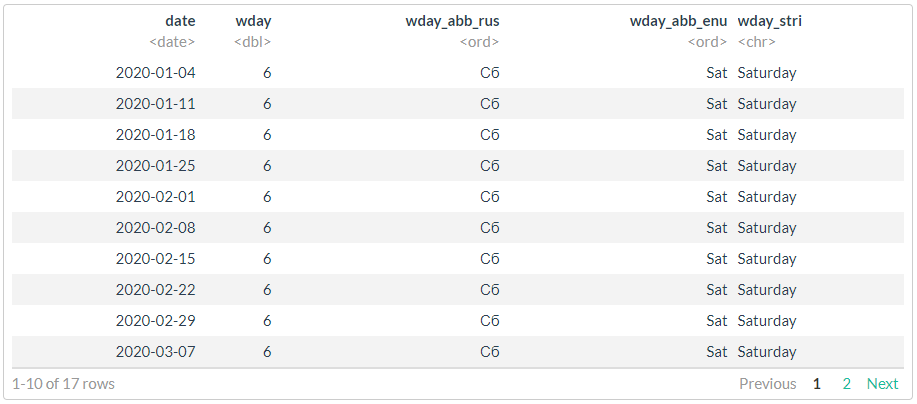
Código de muestra. No olvide que una serie de funciones funcionan teniendo en cuenta la configuración regional de la máquina en la que se ejecuta el código. Y si su mes está impreso en ruso, entonces esto no garantiza (si no usa métodos) un comportamiento similar en otra máquina u otro sistema operativo.
# https://stackoverflow.com/questions/16347731/how-to-change-the-locale-of-r
# https://jangorecki.gitlab.io/data.cube/library/stringi/html/stringi-locale.html
df <- as.Date("2020-01-01") %>%
seq.Date(to = . + months(4), by = "1 day") %>%
tibble(date = .) %>%
mutate(wday = lubridate::wday(date, week_start = 1),
wday_abb_rus = lubridate::wday(date, label = TRUE, week_start = 1),
wday_abb_enu = lubridate::wday(date, label = TRUE, week_start = 1, locale = "English"),
wday_stri = stringi::stri_datetime_format(date, "EEEE", locale = "en"))
#
filter(df, wday == 6)
PD: La mayoría de las pruebas son solo por ejemplo. Puede ejecutarlo en sus máquinas, los números serán completamente diferentes, pero la naturaleza de la dependencia y la proporción deben ser aproximadamente las mismas.
Entrada anterior - "R vs Python en un ciclo productivo" .