
En este artículo se analiza la competencia de aprendizaje automático Riesgo de incumplimiento crediticio de la vivienda , cuyo objetivo es utilizar datos históricos sobre solicitudes de préstamo para predecir si un solicitante podrá pagar un préstamo (determinar el riesgo de incumplimiento de un prestatario). Predecir si un cliente pagará un préstamo o tendrá problemas es un desafío comercial crítico, y Home Credit está organizando una competencia en la plataforma Kaggle para ver qué modelos de aprendizaje automático puede desarrollar la comunidad para ayudarlos con este desafío.
Esta es una tarea de clasificación supervisada estándar:
Aprendizaje supervisado: las respuestas correctas se incluyen en los datos de entrenamiento y el objetivo es entrenar el modelo para predecir estas respuestas en función de las señales disponibles.
: , – 0 ( ) 1 ( ).
Home Credit, () , . 7 :
applicationtrain / applicationtest: Home Credit. , SKIDCURR . TARGET :
0, ;
1, .
bureau: . , .
bureaubalance: . . , .
previousapplication: Home Credit , . , SKIDPREV.
POSCASHBALANCE: , Home Credit. , .
creditcardbalance: , Home Credit. . .
installments_payment: Home Credit, .
, :

, ( HomeCredit_columns_description.csv) .
(application_train / application_test), . , . , ! - , .
: ROC AUC
( ), , . , (ROC AUC, AUROC).
ROC AUC , , .
(ROC) , , , , :
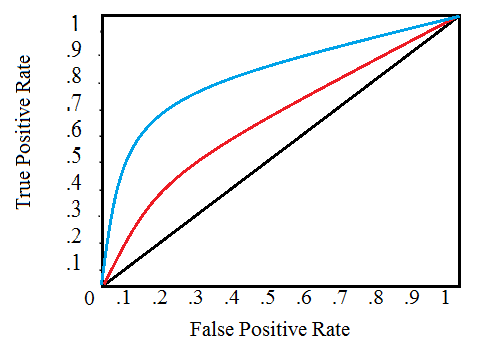
, , . 0 1 . , , . , , , , , , ( ).
(AUC) . ROC ( ). 0 1, . , , ROC AUC = 0,5.
ROC AUC, 0 1, 0 1. , , , ( , ) — . , , 99,9999%, , , . , ( ), , ROC AUC F1, . ROC AUC , ROC AUC .
, , . , , . .
: numpy pandas , sklearn preprocessing , matplotlib ¨C11C¨C12C¨C13C . .
import os
import numpy as np
import pandas as pd
pd.set_option('display.max_columns', None)
from sklearn.preprocessing import LabelEncoder
import matplotlib.pyplot as plt
import seaborn as sns
#
import warnings
warnings.filterwarnings('ignore')
, , . 9 : ( ), ( ), 6 , .
#
print(os.listdir("../input/"))
‘POSCASHbalance.csv’, ‘bureaubalance.csv’, ‘applicationtrain.csv’, ‘previousapplication.csv’, ‘installmentspayments.csv’, ‘creditcardbalance.csv’, ‘samplesubmission.csv’, ‘applicationtest.csv’, ‘bureau.csv’]
#
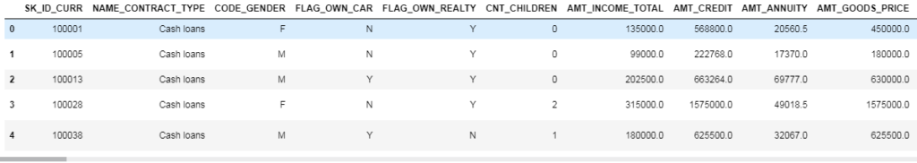
app_train = pd.read_csv('../input/application_train.csv')
print('Training data shape: ', app_train.shape)
app_train.head()
Training data shape: (307511, 122)

307511 , 120 , , .
#
app_test = pd.read_csv('../input/application_test.csv')
print('Testing data shape: ', app_test.shape)
app_test.head()
Testing data shape: (48744, 121)
, TARGET.
(EXPLORATORY DATA ANALYSIS – EDA)
(EDA) — , , , , . EDA — , . , , . , , , , .
— , : 0, , 1, . , .
app_train['TARGET'].value_counts()

app_train['TARGET'].astype(int).plot.hist();
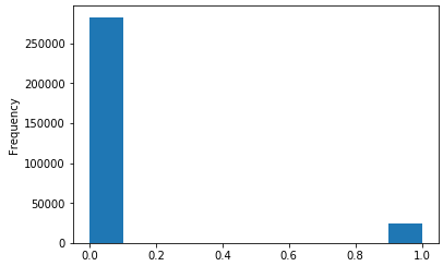
.
#
def missing_values_table(df):
#
mis_val = df.isnull().sum()
#
mis_val_percent = 100 * df.isnull().sum() / len(df)
#
mis_val_table = pd.concat([mis_val, mis_val_percent], axis=1)
#
mis_val_table_ren_columns = mis_val_table.rename(
columns = {0 : 'Missing Values', 1 : '% of Total Values'})
#
mis_val_table_ren_columns = mis_val_table_ren_columns[
mis_val_table_ren_columns.iloc[:,1] != 0].sort_values(
'% of Total Values', ascending=False).round(1)
#
print("Your selected dataframe has " + str(df.shape[1]) + " columns.\n"
"There are " + str(mis_val_table_ren_columns.shape[0]) +
" columns that have missing values.")
return mis_val_table_ren_columns
#
missing_values = missing_values_table(app_train)
missing_values.head(10)
Your selected dataframe has 122 columns.
There are 67 columns that have missing values.

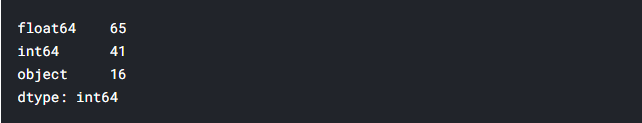
. int64 float64 — ( ). object .
#
app_train.dtypes.value_counts()
object().
#
app_train.select_dtypes('object').apply(pd.Series.nunique, axis = 0)

, . .
, . , ( , LightGBM). , () , . :
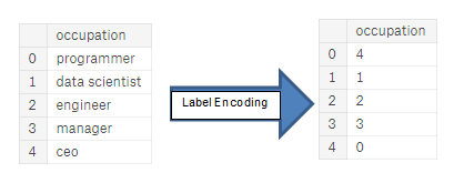
(Label encoding): . . :
(One-hot encoding): . 1 0 .

, . , , - . 4, — 1, , . . , , (, = 4 = 1) , , . (, / ), , .
, , . – Kaggle-master Will Koehrsen, , , . . , ( ) - . , PCA , ( , ).
Label Encoding 2 One-Hot Encoding 2 . , , , , . - .
Label Encoding One-Hot Encoding
: (dtype == object) , – .
LabelEncoder Scikit-Learn, – pandas get_dummies(df).
# label encoder
le = LabelEncoder()
le_count = 0
#
for col in app_train:
if app_train[col].dtype == 'object':
# 2
if len(list(app_train[col].unique())) <= 2:
# LabelEncoder
le.fit(app_train[col])
#
app_train[col] = le.transform(app_train[col])
app_test[col] = le.transform(app_test[col])
# , LabelEncoder
le_count += 1
print('%d columns were label encoded.' % le_count)
3 columns were label encoded.
# one-hot encoding
app_train = pd.get_dummies(app_train)
app_test = pd.get_dummies(app_test)
print('Training Features shape: ', app_train.shape)
print('Testing Features shape: ', app_test.shape)
raining Features shape: (307511, 243)
Testing Features shape: (48744, 239).
(). , , . . ( , ). , axis = 1, , !
train_labels = app_train['TARGET']
# , ,
app_train, app_test = app_train.align(app_test, join = 'inner', axis = 1)
#
app_train['TARGET'] = train_labels
print('Training Features shape: ', app_train.shape)
print('Testing Features shape: ', app_test.shape)
Training Features shape: (307511, 240)
Testing Features shape: (48744, 239)
, . «» . - , , ( , ), .
, EDA, — . - , , . describe. DAYS_BIRTH , . , -1 :
(app_train['DAYS_BIRTH'] / -365).describe()

— . .
app_train['DAYS_EMPLOYED'].describe()
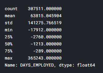
– ( , ) — 1000 !
app_train['DAYS_EMPLOYED'].plot.hist(title = 'Days Employment Histogram');
plt.xlabel('Days Employment');
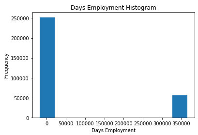
, .
anom = app_train[app_train['DAYS_EMPLOYED'] == 365243]
non_anom = app_train[app_train['DAYS_EMPLOYED'] != 365243]
print('The non-anomalies default on %0.2f%% of loans' % (100 * non_anom['TARGET'].mean()))
print('The anomalies default on %0.2f%% of loans' % (100 * anom['TARGET'].mean()))
print('There are %d anomalous days of employment' % len(anom))
The non-anomalies default on 8.66% of loans
The anomalies default on 5.40% of loans
There are 55374 anomalous days of employment
– , .
. — , . , , , - . , , , . (np.nan), , , .
# ,
app_train['DAYS_EMPLOYED_ANOM'] = app_train["DAYS_EMPLOYED"] == 365243
# nan
app_train['DAYS_EMPLOYED'].replace({365243: np.nan}, inplace = True)
app_train['DAYS_EMPLOYED'].plot.hist(title = 'Days Employment Histogram');
plt.xlabel('Days Employment');

, . , , ( nans , , ). DAYS , , .
: , , . np.nan .
app_test['DAYS_EMPLOYED_ANOM'] = app_test["DAYS_EMPLOYED"] == 365243
app_test["DAYS_EMPLOYED"].replace({365243: np.nan}, inplace = True)
print('There are %d anomalies in the test data out of %d entries' % (app_test["DAYS_EMPLOYED_ANOM"].sum(), len(app_test)))
There are 9274 anomalies in the test data out of 48744 entries
, , EDA. — . , .corr.
.00–0.19 « »
.20-.39 «»
.40–0.59 «»
0,60–0,79 «»
0,80–1,0 « »
#
correlations = app_train.corr()['TARGET'].sort_values()
#
print('Most Positive Correlations:\n', correlations.tail(15))
print('\nMost Negative Correlations:\n', correlations.head(15))
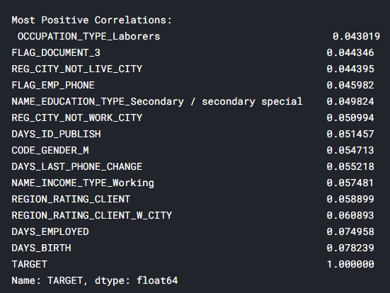
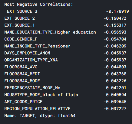
: DAYSBIRTH — ( TARGET, 1). , DAYSBIRTH — . , , , , , (.. == 0). , , .
app_train['DAYS_BIRTH'] = abs(app_train['DAYS_BIRTH'])
app_train['DAYS_BIRTH'].corr(app_train['TARGET'])
-0.07823930830982694
, , , , .
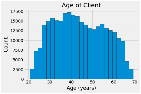
. -, . , x .
plt.style.use('fivethirtyeight')
#
plt.hist(app_train['DAYS_BIRTH'] / 365, edgecolor = 'k', bins = 25)
plt.title('Age of Client'); plt.xlabel('Age (years)'); plt.ylabel('Count');
, , , . , (KDE), . ( , , , ). seaborn kdeplot.
plt.figure(figsize = (10, 8))
sns.kdeplot(app_train.loc[app_train['TARGET'] == 0, 'DAYS_BIRTH'] / 365, label = 'target == 0')
sns.kdeplot(app_train.loc[app_train['TARGET'] == 1, 'DAYS_BIRTH'] / 365, label = 'target == 1')
plt.xlabel('Age (years)'); plt.ylabel('Density'); plt.title('Distribution of Ages');
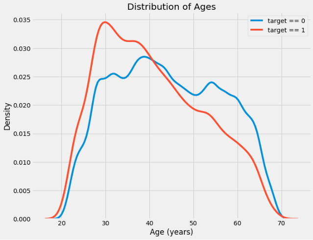
target == 1 . ( -0,07), , , , . : .
, 5 . , .
age_data = app_train[['TARGET', 'DAYS_BIRTH']]
age_data['YEARS_BIRTH'] = age_data['DAYS_BIRTH'] / 365
age_data['YEARS_BINNED'] = pd.cut(age_data['YEARS_BIRTH'], bins = np.linspace(20, 70, num = 11))
age_data.head(10)

#
age_groups = age_data.groupby('YEARS_BINNED').mean()
age_groups

plt.figure(figsize = (8, 8))
plt.bar(age_groups.index.astype(str), 100 * age_groups['TARGET'])
plt.xticks(rotation = 75); plt.xlabel('Age Group (years)'); plt.ylabel('Failure to Repay (%)')
plt.title('Failure to Repay by Age Group');

: . 10% 5% .
: , , . , , , .
: EXTSOURCE1, EXTSOURCE2 EXTSOURCE3. , « ». , , , , , .
.
-, EXT_SOURCE .
ext_data = app_train[['TARGET', 'EXT_SOURCE_1', 'EXT_SOURCE_2', 'EXT_SOURCE_3', 'DAYS_BIRTH']]
ext_data_corrs = ext_data.corr()
ext_data_corrs

plt.figure(figsize = (8, 6))
#
sns.heatmap(ext_data_corrs, cmap = plt.cm.RdYlBu_r, vmin = -0.25, annot = True, vmax = 0.6)
plt.title('Correlation Heatmap');
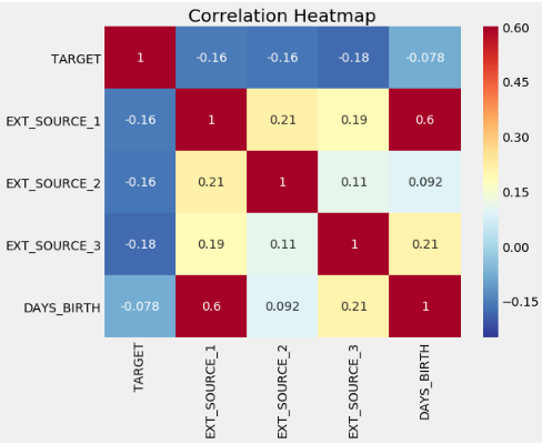
EXT_SOURCE , , EXT_SOURCE . , DAYS_BIRTH EXT_SOURCE_1, , , , .
, . .
plt.figure(figsize = (10, 12))
for i, source in enumerate(['EXT_SOURCE_1', 'EXT_SOURCE_2', 'EXT_SOURCE_3']):
plt.subplot(3, 1, i + 1)
sns.kdeplot(app_train.loc[app_train['TARGET'] == 0, source], label = 'target == 0')
sns.kdeplot(app_train.loc[app_train['TARGET'] == 1, source], label = 'target == 1')
plt.title('Distribution of %s by Target Value' % source)
plt.xlabel('%s' % source); plt.ylabel('Density');
plt.tight_layout(h_pad = 2.5)
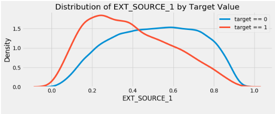
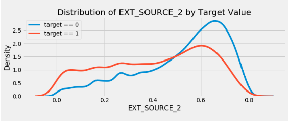
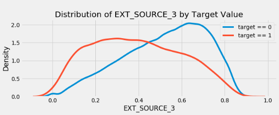
EXT_SOURCE_3 . , . ( ), , , .
EXTSOURCE DAYSBIRTH. – , , . seaborn PairGrid, , 2D .
plot_data = ext_data.drop(columns = ['DAYS_BIRTH']).copy()
plot_data['YEARS_BIRTH'] = age_data['YEARS_BIRTH']
plot_data = plot_data.dropna().loc[:100000, :]
#
def corr_func(x, y, **kwargs):
r = np.corrcoef(x, y)[0][1]
ax = plt.gca()
ax.annotate("r = {:.2f}".format(r),
xy=(.2, .8), xycoords=ax.transAxes,
size = 20)
#
grid = sns.PairGrid(data = plot_data, size = 3, diag_sharey=False,
hue = 'TARGET',
vars = [x for x in list(plot_data.columns) if x != 'TARGET'])
grid.map_upper(plt.scatter, alpha = 0.2)
grid.map_diag(sns.kdeplot)
grid.map_lower(sns.kdeplot, cmap = plt.cm.OrRd_r);
plt.suptitle('Ext Source and Age Features Pairs Plot', size = 32, y = 1.05);
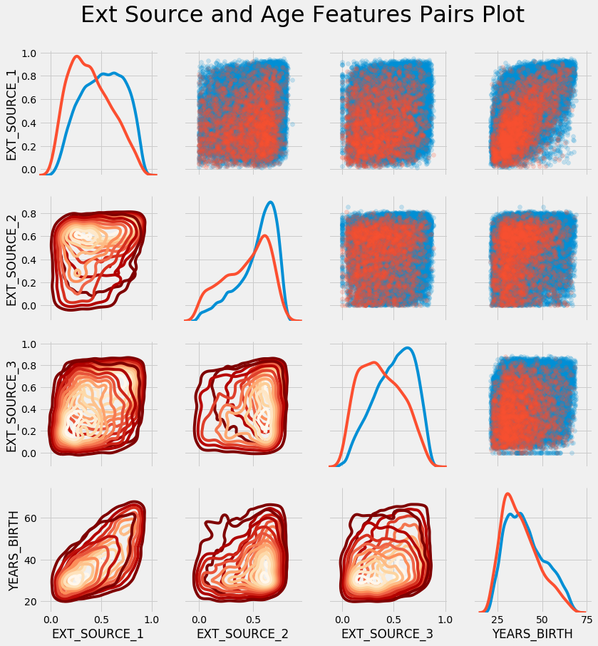
En este gráfico, el rojo indica los préstamos que no se han reembolsado y el azul indica los préstamos que se han reembolsado. Podemos ver varias relaciones en los datos. De hecho, existe una relación lineal positiva moderada entre EXT_SOURCE_1 y YEARS_BIRTH, lo que indica que este rasgo puede estar relacionado con la edad.
Con esto concluye el primer artículo. En la siguiente parte, hablaré sobre el desarrollo de funciones adicionales basadas en los datos disponibles y también demostraré cómo crear un modelo simple de aprendizaje automático.
En la preparación del artículo se utilizaron materiales de fuentes abiertas: source_1 , source_2 .