
En lugar de un epílogo
Esta historia sucedió hace bastante tiempo, pero algunos de los detalles se han aclarado solo ahora, por lo que ha llegado el momento de contarlo.
No nos detendremos en la descripción de los tipos de realidades paralelas, esto se ha hecho durante mucho tiempo y con éxito por muchos escritores, fanáticos de la historia alternativa, futuristas y simplemente fanáticos de tales cosas. Vayamos directo al grano.
, . ., «» . , . . : « :
1) 1000 ;
2) .1 , .
« » , . , .
. : « » . . , .. notebook c Anaconda. , ython , .
, 1000 . , , , 1 . : « » « ».
:
#
# Pivot :
Cnt_arr = pd.DataFrame()
Cnt_arr = F_Lst_FULL_df.pivot_table('DT_evnt', index='Date_event',dropna = False,fill_value=0, columns='Type',aggfunc='count')
#
sns.set() # seaborn styles
Cnt_arr.plot()
plt.xlabel(' ')
plt.ylabel(' ')
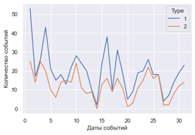
. , . . , — =1, , =2 .
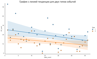
« . » — , « , , – ?».
5 :
#
sns.set_style("white")
gridobj = sns.lmplot(x='Date_event', y='DT_evnt', hue='Type', data=Cnt_arr, height=7, aspect=1.6,
robust=True, palette='tab10', scatter_kws=dict(s=60, linewidths=.7, edgecolors='black'))
# !
# : 0-100!
# X (min, max)
Xmin=Cnt_arr['Date_event'].min()-1
Xmax=Cnt_arr['Date_event'].max()+1
# Y (min, max)
Ymin=Cnt_arr['DT_evnt'].min()-1
Ymax=Cnt_arr['DT_evnt'].max()+1
#
gridobj.set(xlim=(Xmin, Xmax), ylim=(Ymin, Ymax))
plt.title(" ",
fontsize=20)
plt.show()
« . !» — , . : « ? , ?».
(, , ), : « , : 1) , ; 2) , .. .»
, , : « . »:
#
# ( )
F_Lst_FULL_df['Date_event'] = F_Lst_FULL_df['DT_evnt']-F_Lst_FULL_df['DT_evnt']%1
# 0 1-
F_Lst_FULL_df['Date_event'] = F_Lst_FULL_df['Date_event'].replace(0.0, 1.0)
# 0 1
F_Lst_FULL_df['PartOfDay'] = F_Lst_FULL_df['DT_evnt']%1
#
F_Lst_FULL_df['NWeek'] = F_Lst_FULL_df['Date_event']//7%7+1
# 1-
F_Lst_FULL_df['D_Week'] = 1 + (F_Lst_FULL_df['Date_event']+6)%7
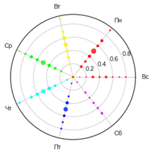
«» . «» « », :
#
# :
# () - , ,
# - pivot
vis_date = F_Lst_FULL_df.pivot_table('DT_evnt', index=['D_Week','PartOfDay'],
dropna = False,fill_value=0, aggfunc='count').reset_index()
Angle_dim = vis_date['D_Week'] #
Radius_dim = vis_date['PartOfDay'] # (0-1) 24
#
#
theta = 2 * np.pi * Angle_dim/7 # Pi (3.14159265...)
#
area = vis_date['DT_evnt'] #
colors = theta # (1-,2-,3-...7-)
fig = plt.figure()
# , :
# : , 111 - , ( ) Figure.
ax = fig.add_subplot(111, projection='polar')
# , ( )
# , !
xtks = pd.DataFrame()
xtks['val']=(2 * np.pi * Angle_dim/7).unique() #
xtks['mrk']=['','','','','','',''] #
plt.xticks(xtks['val'].tolist(),xtks['mrk'].tolist())
c = ax.scatter(theta, Radius_dim, c=colors, s=area, cmap='hsv', alpha=0.75)
« – , » — , . « . ?» — , . « » — .
, :
# ( 0-1)
d = preprocessing.normalize(F_Lst_FULL_df,axis=0)
scaled_df = pd.DataFrame(d,columns = ['DT_evnt', 'Type', 'Date_event', 'PartOfDay','NWeek','D_Week'])
del d
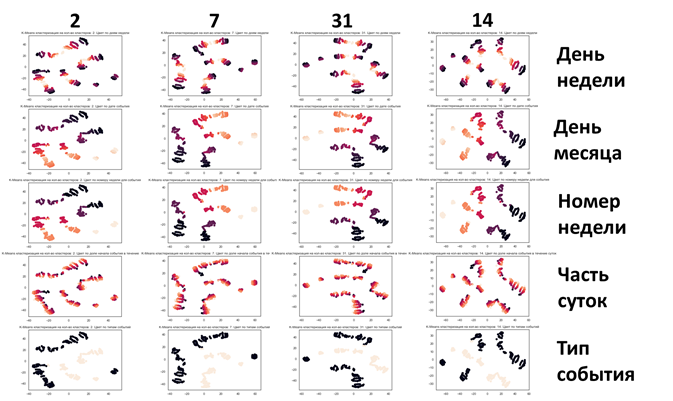
(k-Menas)
: «N_Clstr .
N_Clstr=2 (/);
N_Clstr=7 ;
N_Clstr=31 ;
N_Clstr=14 .»
#
N_Clstr=14
model = KMeans(n_clusters=N_Clstr)
#
model.fit(scaled_df)
#
all_predictions = model.predict(scaled_df)
( )
«», . . « TSNE 2D.
#
model = TSNE()
#
transformed = model.fit_transform(scaled_df)
#
x_axis = transformed[:, 0]
y_axis = transformed[:, 1]
, ,
plt.title('K-Means - : '+str(N_Clstr)+'. ')
plt.scatter(x_axis, y_axis, c=scaled_df['Type'])
plt.show()
# :
# D_Week
# PartOfDay
# Date_event
# NWeek
, , : «, , , , ( ), - ( ( ).
:
1) ,
2) .
, «» . , !».
Vibegallo se mostró muy complacido, sonriendo ampliamente, preguntó: "¿Ya se publicó el informe?" "Por supuesto, todos estos datos están aquí". Alexander sacó una carpeta del cajón superior.
"¡Estás bien hecho! ¡Definitivamente te marcaré al resumir los resultados del año! " - dijo Vibegallo y se dirigió resueltamente a la secretaría de la Troika.