¡Hola Habr! Por mi profesión principal soy ingeniero para el desarrollo de campos de petróleo y gas. Me estoy sumergiendo en Data Sciense y esta es mi primera publicación en la que me gustaría compartir mi experiencia con el aprendizaje automático en la industria petrolera.

. , , .
. , ( ).
, . .
:
( + ) () () , .
( ). () . , , - - , .
, , . .
3D ().
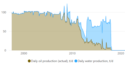
, ( ). . , . . . . 10 - 15 . , 3- 250 - 1000 . , , " ".
. . . - , . - 3- ( , ) ( ). . , .
. .
:
( , , /- , , ..),
- , , .
. . , . , . , - . .. Q/(Q + Q)*100%
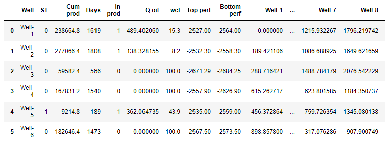
( ) :
:
Cum oil:
Days: ( ( ) ).
In prod: /
Q oil:
wct:
Top perf: -
Bottom perf:
ST: 0 - , 1 -
x, y:
import numpy as np
import pandas as pd
import matplotlib.pyplot as plt
%matplotlib inline
%config InlineBackend.figure_format = 'svg'
import pylab
from pylab import rcParams
import plotly.express as px
import plotly.graph_objects as go
from sklearn.model_selection import train_test_split
from sklearn.ensemble import RandomForestRegressor
from sklearn.metrics import r2_score as r2, mean_absolute_error as mae, mean_squared_error as mse, accuracy_score
from sklearn.metrics.pairwise import euclidean_distances
.
data_path = 'art_df.xlsx'
df = pd.read_excel(data_path, sheet_name='artificial')
df

- . ( ).
ax = df.plot(kind='scatter', x='x', y='y')
df[['x','y','Well']].apply(lambda row: ax.text(*row),axis=1);
rcParams['figure.figsize'] = [11, 8]
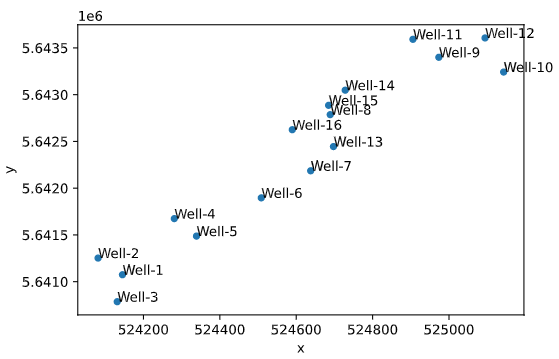
, " " . . , , .
.
distance = pd.DataFrame(euclidean_distances(df[['x', 'y']]))
distance
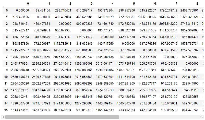
. .
well_names = df['Well']
distance.columns = well_names
. - , .
df_distance = pd.concat([df.drop(['x', 'y'], axis=1), distance], axis=1)
df_distance
. , ,
df_train_1 = df_distance.drop([12, 13, 14, 15], axis=0)
df_train_1

df_test_1 = df_distance.loc[[12, 13]]
df_test_1

DataFrame X_1. ( ) wct.
x_1 = df_train_1.drop(['Well', 'wct'], axis=1)
x_1

y_1
y_1 = df_train_1['wct']
y_test_1
y_test_1 = df_test_1['wct']
Random Forest Reggressor, , .
x_test_1 = df_test_1.drop(['Well', 'wct'], axis=1)
model = RandomForestRegressor(random_state=42, max_depth=14)
model.fit(x_1, y_1)
y_pred_train_1 = model.predict(x_1)
y_pred_1 = model.predict(x_test_1)
print('Predicted values from train data:')
r2_train = r2(y_1, y_pred_train_1)
mae_train = mae(y_1, y_pred_train_1)
mse_train = mse(y_1, y_pred_train_1)
print(f'R2 train: {r2_train.round(4)}')
print(f'MAE train: {mae_train.round(4)}')
print(f'MSE train: {mse_train.round(4)}')
print('Predicted values from test data:')
r2_test = r2(y_test_1, y_pred_1)
mae_test = mae(y_test_1, y_pred_1)
mse_test = mse(y_test_1, y_pred_1)
print(f'R2 test: {r2_test.round(4)}')
print(f'MAE test: {mae_test.round(4)}')
print(f'MSE test: {mse_test.round(4)}')
model
Predicted values from train data:
R2 train: 0.8832
MAE train: 8.2855
MSE train: 131.1208
Predicted values from test data:
R2 test: 0.8758
MAE test: 3.164
MSE test: 11.4485
RandomForestRegressor(max_depth=14, random_state=42)
R2 R2 1%. , .
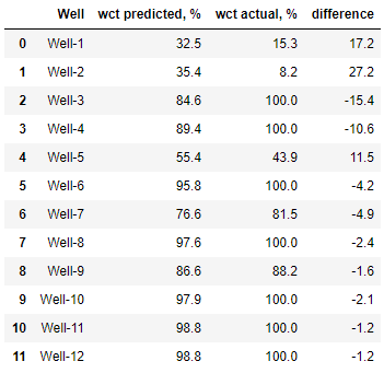
, (blind test)
df_y_test = pd.DataFrame({'Well': df_test_1['Well'],
'wct predicted, %': y_pred_1.round(1),
'wct actual, %': y_test_1.round(1),
'difference': (y_pred_1 - y_test_1).round(1)})
df_y_test

df_y_train = pd.DataFrame({'Well': df_train_1['Well'],
'wct predicted, %': y_pred_train_1.round(1),
'wct actual, %': y_1.round(1),
'difference': (y_pred_train_1 - y_1).round(1)})
df_y_train
:
round(sum(abs(y_pred_train_1 - y_1)) / len(y_1), 1)
8.3
, 8%, .
, ,
df_train_2 = df_distance.drop([14, 15], axis=0)
, .
WCT () = NaN.
df_fc = df_distance.loc[[14, 15]]
DataFrame x_2. ( ) wct.
x_2 = df_train_2.drop(['Well', 'wct'], axis=1)
y_2 .
y_2 = df_train_2['wct']
x_fc = df_fc.drop(['Well', 'wct'], axis=1)
model = RandomForestRegressor(random_state=42, max_depth=14)
model.fit(x_2, y_2)
y_pred_train_2 = model.predict(x_2)
y_fc = model.predict(x_fc)
print('Predicted values from train data:')
r2_train = r2(y_2, y_pred_train_2)
mae_train = mae(y_2, y_pred_train_2)
mse_train = mse(y_2, y_pred_train_2)
print(f'R2 train: {r2_train.round(4)}')
print(f'MAE train: {mae_train.round(4)}')
print(f'MSE train: {mse_train.round(4)}')
print('Forecasted values could be compared with real data!')
model
Predicted values from train data:
R2 train: 0.9095
MAE train: 6.5196
MSE train: 89.9625
RandomForestRegressor(max_depth=14, random_state=42)
R2 .
.
df_y_train = pd.DataFrame({'Well': df_train_2['Well'],
'wct predicted, %': y_pred_train_2.round(1),
'wct actual, %': y_2.round(1),
'difference': (y_pred_train_2 - y_2).round(1)})
df_y_train
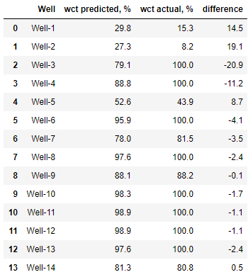
round(sum(abs(y_pred_train_2 - y_2)) / len(y_2), 1)
6,5
6,5. !
:
df_y_test = pd.DataFrame({'Well': df_test_1['Well'],
'wct predicted, %': y_pred_1.round(1),
'wct actual, %': y_test_1.round(1),
'difference': (y_pred_1 - y_test_1).round(1)})
df_y_test

.
model.feature_importances_
feature_importances = pd.DataFrame()
feature_importances['feature_name'] = x_2.columns.tolist()
feature_importances['importance'] = model.feature_importances_
feature_importances = feature_importances.sort_values(by='importance', ascending=False)
feature_importances
fig = px.bar(feature_importances,
x=feature_importances['importance'],
y=feature_importances['feature_name'],
title="Feature importances")
fig.update_layout(yaxis={'categoryorder':'total ascending'})
fig.show()
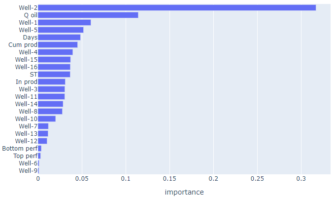
, - 2- . .
. - .
fig = px.scatter(x=y_pred_train_2, y=y_2, title="True vs Predicted values",
text=df_train_2['Well'], width=850, height=800)
fig.add_trace(go.Scatter(x=[0,100], y=[0,100], mode='lines', name='True=Predicted',
line = dict(color='red', width=1, dash='dash')))
fig.update_xaxes(title_text='Predicted')
fig.update_yaxes(title_text='True')
fig.show()

. (- ), (, ).
, " " . , , .
. - "" - .

. " ", . "" . . , .
, . , .
Los datos de pozo no son datos públicos, sino propiedad de la empresa que posee la licencia para desarrollar el campo. Por tanto, para ilustrar el trabajo realizado, se generaron datos de pozos artificiales que están disponibles para este trabajo.
El código fuente junto con el texto del artículo está disponible aquí: https://github.com/alex-kalinichenko/re/tree/master/wct_fc