Muchas personas al menos una vez tuvieron la necesidad de dibujar rápidamente un mapa de una ciudad o país, poniendo sus datos en él (puntos, rutas, mapas de calor, etc.).

Cómo resolver rápidamente ese problema, dónde obtener un mapa de una ciudad o país para dibujar, en las instrucciones detalladas debajo del corte.

Introducción

(, , ) .

, :

, , , , ( , / / ).

, .shp geopandas.

, :

1. —
2. "1"
3. ,

, , , .

Shapefile.

, Shapefile — , (, ), (, ).

, :

• —
• — ,
• — , \

.

OpenStreetMap ( OSM). , — , .

, . OSM.

OSM, ( , ).

NextGis, , .

NextGis ( ~30 ) — ( ~4 ). .

— , ( ) ( / ).

, , (, , , ). , , , , , .

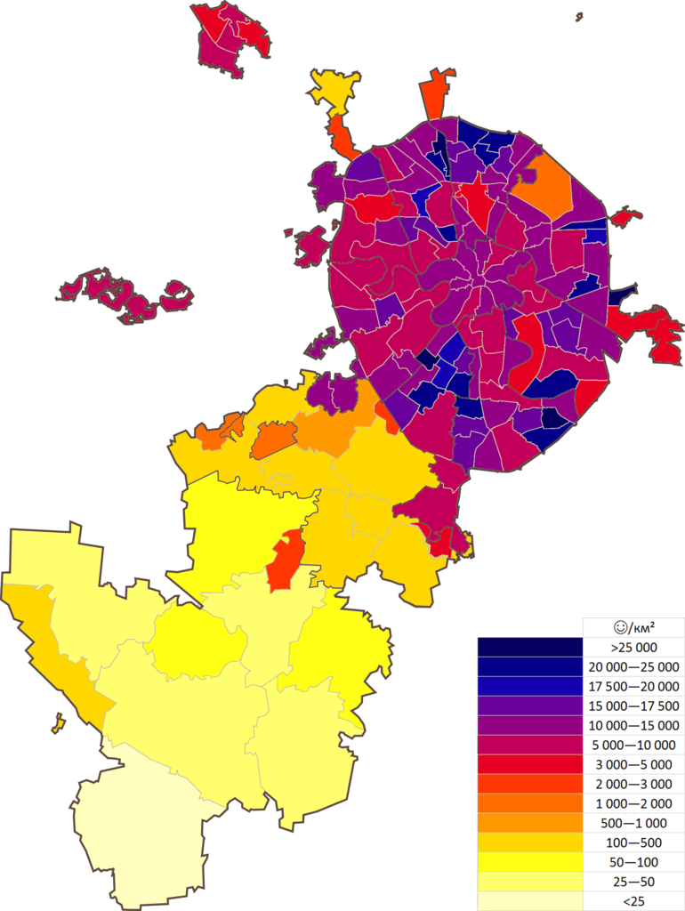
OpenStreetMap. , .

, , , , "".

, . , , , .

, ( "").

, , , !

Geopandas, Pandas, Matplotlib Numpy.

Geopandas pip Windows , conda install geopandas .

import pandas as pd
import numpy as np
import geopandas as gpd
from matplotlib import pyplot as plt

Shapefile

zip .

data . , ( .shp) ( .cpg, .dbf, .prj, .shx).

, geopandas:

• . , 1.2GB, 22.8GB. , — ( geopandas )
• . , 'cp1251', — 'utf-8'
• , , - . .

#    data   
#       zip-     
ZIP_PATH = 'zip://C:/Users/.../Moscow.zip!data/'

#        shp 
LAYERS_DICT = {
    'boundary_L2': 'boundary-polygon-lvl2.shp', #    
    'boundary_L4': 'boundary-polygon-lvl4.shp',
    'boundary_L5': 'boundary-polygon-lvl5.shp',
    'boundary_L8': 'boundary-polygon-lvl8.shp',
    'building_point': 'building-point.shp',  # ,    
    'building_poly': 'building-polygon.shp'  # ,    
              }

#        
i = 0
for layer in LAYERS_DICT.keys():

    path_to_layer = ZIP_PATH + LAYERS_DICT[layer]

    if layer[:8]=='boundary':
        encoding = 'cp1251'
    else:
        encoding = 'utf-8'
    globals()[layer] = gpd.read_file(path_to_layer, encoding=encoding)

    i+=1
    print(f'[{i}/{len(LAYERS_DICT)}] LOADED {layer} WITH ENCODING {encoding}')

:

[1/6] LOADED boundary_L2 WITH ENCODING cp1251
[2/6] LOADED boundary_L4 WITH ENCODING cp1251
[3/6] LOADED boundary_L5 WITH ENCODING cp1251
[4/6] LOADED boundary_L8 WITH ENCODING cp1251
[5/6] LOADED building_point WITH ENCODING utf-8
[6/6] LOADED building_poly WITH ENCODING utf-8

GeoDataFrame, . :

fig, (ax1, ax2, ax3, ax4) = plt.subplots(1, 4, figsize=(15,15))
boundary_L2.plot(ax=ax1, color='white', edgecolor='black')
boundary_L4.plot(ax=ax2, color='white', edgecolor='black')
boundary_L5.plot(ax=ax3, color='white', edgecolor='black')
boundary_L8.plot(ax=ax4, color='white', edgecolor='black')

, , OSM. — .

. - , .

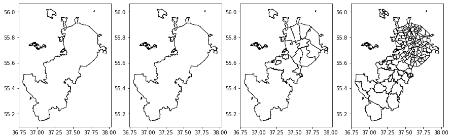
building_poly.plot(figsize=(10,10))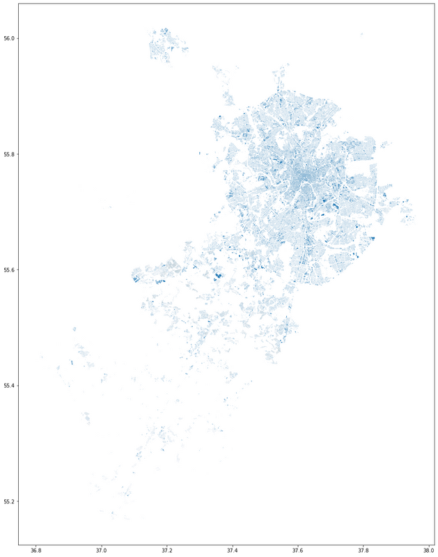

:

base = boundary_L2.plot(color='white', alpha=.8, edgecolor='black', figsize=(50,50))
boundary_L8.plot(ax=base, color='white', edgecolor='red', zorder=-1)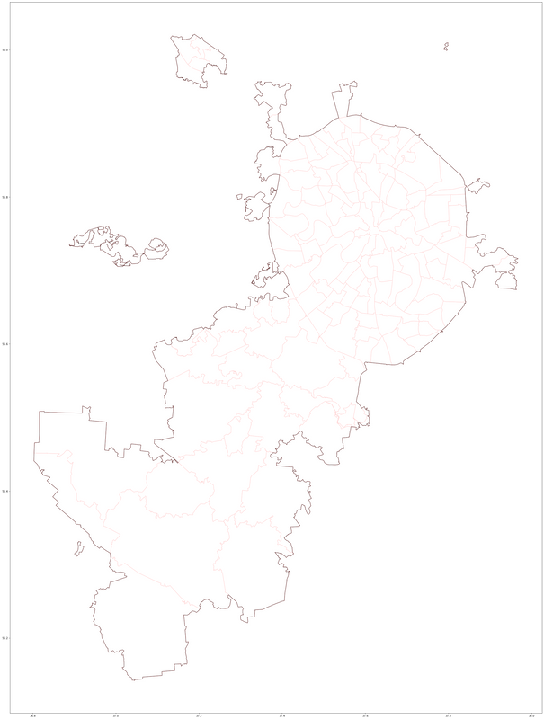

gpd.

, Geopandas Pandas. , (, ), , .

boundary_L8.head()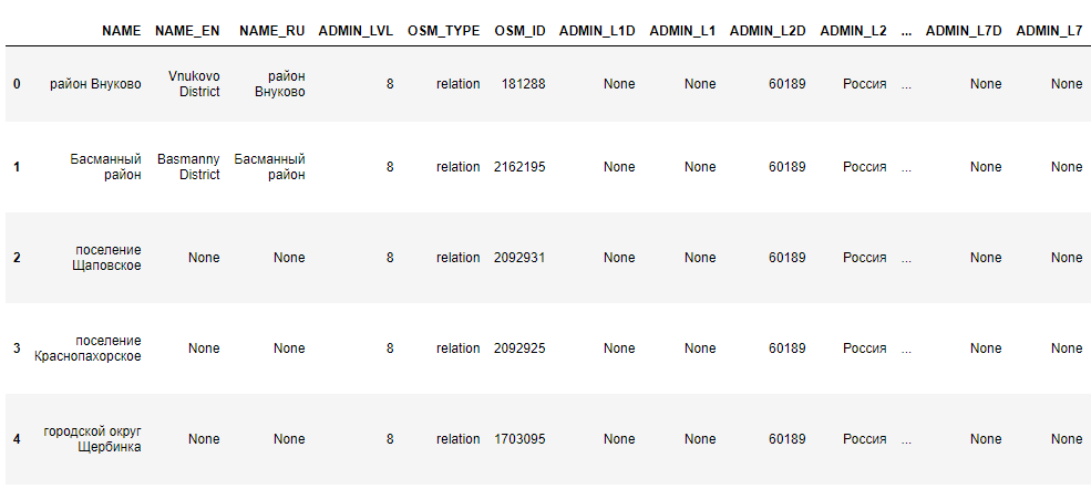

2:

• OSM_ID — OpenStreetMap
• geometry —

.

, , :

print('POLYGONS')
print('# buildings total', building_poly.shape[0])
building_poly = building_poly.loc[building_poly['A_PSTCD'].notna()]
print('# buildings with postcodes', building_poly.shape[0])
print('\nPOINTS')
print('# buildings total', building_point.shape[0])
building_point = building_point.loc[building_point['A_PSTCD'].notna()]
print('# buildings with postcodes', building_point.shape[0])

:

POLYGONS
# buildings total 241511
# buildings with postcodes 13198

POINTS
# buildings total 1253
# buildings with postcodes 4

, , ( , 5%, 13 ).

:

2. OSM-ID ,
3. , "" . , , .

%%time
building_areas = gpd.GeoDataFrame(building_poly[['A_PSTCD', 'geometry']])
building_areas['area'] = 'NF'

#     ,         

#      ,          .centroid.
#      ,      

for area in boundary_L8['OSM_ID']: 
    area_geo = boundary_L8.loc[boundary_L8['OSM_ID']==area, 'geometry'].iloc[0]
    nf_buildings = building_areas['area']=='NF' #       ,      
    building_areas.loc[nf_buildings, 'area'] = np.where(building_areas.loc[nf_buildings, 'geometry'].centroid.within(area_geo), area, 'NF')

#  ,     ,    -  .
#       ,      .
codes_pivot = pd.pivot_table(building_areas,
                             index='A_PSTCD',
                             columns='area',
                             values='geometry',
                             aggfunc=np.count_nonzero)

#  ,           
codes_pivot['main_area'] = codes_pivot.idxmax(axis=1)

#       ""   
for pst_code in codes_pivot.index:
    main_area = codes_pivot.loc[codes_pivot.index==pst_code, 'main_area']
    share = codes_pivot.loc[codes_pivot.index==pst_code, main_area].iloc[0,0] / codes_pivot.loc[codes_pivot.index==pst_code].sum(axis=1)*100
    codes_pivot.loc[codes_pivot.index==pst_code, 'share_in_main_area'] = int(share)

#     
codes_pivot = codes_pivot.loc[:, ['main_area', 'share_in_main_area']].fillna(0)

:

, , , , ( , ).

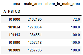
: "1".

#     - 
codes_pivot['count_1'] = codes_pivot.index.str.count('1')
#      
areas_pivot = pd.pivot_table(codes_pivot, index='main_area', values='count_1', aggfunc=np.mean)
areas_pivot.index = areas_pivot.index.astype('int64')
#        
boundary_L8_w_count = boundary_L8.merge(areas_pivot, how='left', left_on='OSM_ID', right_index=True)
#   
boundary_L8_w_count.plot(column='count_1', legend=True, figsize=(10,10))

:

, — ,

, , , .

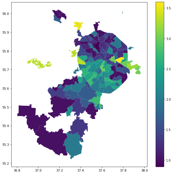
— share_in_main_area

, "" :

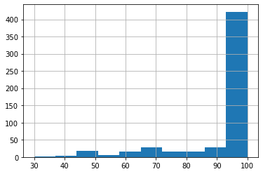
codes_pivot[codes_pivot['share_in_main_area']>50].shape[0]/codes_pivot.shape[0]

:

0.9568345323741008

.

Geopandas — . Matplotlib Pandas .

OSM — , .

, !

— .